Modeling of flow of two-phase mixture in curved channel pipeline

1. Introduction

According to studies hydrocarbon hydrates are white crystalline solids, like snow, and at seal similar to ice [1]. The condensed phase in the flow of natural gas hydrates in addition may contain other solid impurities (slag, sand, etc.) Mechanical impact at high velocity a mixture of gas and particles can be exposed structural elements and stop measuring gas equipment. Assessment of the impact can be made on the basis of solving the equations of motion of a two-phase mixture in the pipeline elements.

2. The equations of two-phase flow of gas in the curved pipes

The system of equations describing the steady flow of viscous heat-conducting gas in an arbitrary coordinate system is as follows:

where $\rho$ – density of the gas; $\mathbf{V}$ – The velocity vector; $e$ – Specific internal energy; $\mathbf{P}$ – Pressure tensor related to pressure $p$ and viscous stress tensor $\mathbf{S}$ relation $\mathbf{P}=p\mathbf{I}+\mathbf{S}$. The viscous stress tensor is defined as:

where $\mathbf{I}$ – the unit tensor, $\mu$ – dynamic viscosity coefficient. Tensor components $\mathbf{S}$ are shown in many literatures, for example in [2]. Heat flow $\mathbf{q}$ is determined by the Fourier law: $\mathbf{q}=-\lambda \nabla T$, where $\lambda$ – coefficient of thermal conductivity, $T$ – temperature. For the system of Eq. (2), you must add the equation of state of the gas in the form $p=\rho RT$, where $R$ – the gas constant. In the calculation of flows with low speeds (up to Mach numbers $M<\text{0.3}$), it is advisable to consider for incompressible. In this case, in the Eq. (1) $\rho =const$ and the equation for the energy can not be seen due to the small change in the flow temperature.

Together with the Eq. (1) it is necessary to solve the equation for the turbulent viscosity. It was used model of turbulent viscosity [3].

The equation for the turbulent viscosity is as follows:

where ${\nu }_T$ – turbulent viscosity; $\mu =\rho ({\nu }_T+{\nu }_0)$, ${\mathrm{\Gamma }}_T$ – A term describing the generation and dissipation of turbulent viscosity [3]; ${\nu }_0$ – Molecular viscosity.

To calculate the flow in curved pipes need to solve the problem of flow in a three-dimensional setting. Solving such problems is difficult enough. To evaluate the mechanical interaction of a condensed phase with the walls will be considered two-dimensional setting. The system of Eqs. (1), (2) can be written in a flat or cylindrical coordinates with axial symmetry ($x$ – longitudinal, $r$ – transverse coordinates). For the curved regions of the flow plane $x$, $r$ applied coordinate transformation taking curvilinear computational domain into a rectangle. The difference mesh is constructed using a complex boundary element method [4].

To write equations used curvilinear orthogonal coordinate $\xi$, $\eta .$ System variables $\xi$, $\eta$ associated with Cartesian coordinates $x$, $r$ as follows: $\xi =\xi (x,r)$, $\eta =\eta (x,r)$. The components of the metric tensor are equal $g_{11}=g_{22}=D$. In the case of orthogonal coordinates $x_{\xi }=r_{\eta }$, $x_{\eta }=-r_{\xi }$, $D=x_{\xi }^2+r_{\xi }^2$.

The equations of continuity, momentum and energy in the coordinate system $\xi$, $\eta$ are of the form [5]:

where $J=\sqrt{D}$; $u$, $v$ – Projections of the velocity vector $\mathbf{v}$ on the axis $\xi$, $\eta$; $E=\rho \left(e+\mathrm{0,5}\cdot V^2\right)$ – the total energy; $T$ – temperature. Axisymmetric flow corresponds to $\gamma =\text{1}$, a flat – $\gamma =\text{0}$. The coefficients in the right sides of the equations in the coordinate system $\xi$, $\eta$ is written as follows:

Odds $Q_1$, $Q_2$, $Q_3$ describe the exchange of momentum and energy between phases:

where, the index $s$ belongs to the dispersed phase; $G$ – The mass evaporation rate drops; $c_s$, ${\rho }_l$ – heat capacity and density of droplets of substance; $n$ – Condensed number of particles per unit volume; $B_u$, $B_T$ – Heat transfer coefficients and the resistance between the phases.

Together with the Eq. (3) it is necessary to solve the equation for the turbulent viscosity. In the plane $x$, $r$ orthogonal difference grid built complex boundary element method.

The basis of the solution of a system of Eq. (3) laid SIMPLE method [6], which is kind of focused on the use of curvilinear coordinates, implemented in [5, 7].

The equations for the dispersed phase is also recorded in a curvilinear coordinate system:

Resistance and heat transfer coefficients are determined by the formulas [6]:

3. The boundary conditions

On the permeable boundaries of the fixed costs of the gas and condensed phase, the enthalpy of the phase and the initial particle size. On impermeable boundaries puts a condition of sticking. At the outlet of the pipe for subsonic and where the pressure was set. On the axis of symmetry – the symmetry condition.

Changing the number n of particles per unit volume is determined by the speed lag of gas (including the interaction of the dispersed phase and gas). We write the equations of momentum and energy transfer:

where ${\varsigma }_s$ – coordinate in the direction from the $s$th path; $W_s=\sqrt{(U_s{)}^2+(V_s{)}^2}$; $U_s=u_s{\xi }_x+v_s{\xi }_r$; $V_s=u_s{\eta }_x+v_s{\eta }_r$; ${\mathbf{f}}_s=(u_s,v_s,T_s)$; ${\mathbf{C}}_s=\left[\begin{array}{l}{A}_{1s}\\ A_{1s}\\ A_{1T}\end{array}\right]$; ${\mathbf{B}}_s=\left[\begin{array}{c}{A}_{1s}u+a_{x}g\\ A_{1s}v+a_{y}g\\ A_{1Ts}T\end{array}\right]\mathrm{}\mathrm{}.$

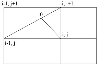
Driving integration of the system Eq. (5) is shown in Fig. 1.

The integration is performed over the interval of the particle trajectory. The segment begins with the diagonal cell comprising an anchor point $\left(i,j\right)$, at 0 particles with known parameters, and ends at the node $(i,j)$, where the parameters to be calculated. To integrate the use of implicit Runge-Kutt second order of approximation:

An index of 0 corresponds to the beginning of the segment of the trajectory. Required parameters ${\phi }_{s0}$ at the point 0 determined by the formula:

using known values ${\phi }_s$ at the ends of the diagonal. The values ${\alpha }_s$, $\mathrm{\Delta }{\varsigma }_s$, $iu$, $jv$ are given by:

The equation for $n_s(\xi ,\eta )$ Eq. (4) is solved by countercurrent scheme [6]. The difference analog of the Eq. (4) has the form:

where $a_{W_{i,j}}=\mathrm{m}\mathrm{a}\mathrm{x}[\delta {\eta }_j{y}_{i-1/2,j}{D}_{i-1/2,j}{U}_{i-1/2,j},0]$, $a_{E_{i,j}}=\mathrm{m}\mathrm{a}\mathrm{x}[-\delta {\eta }_j{y}_{i+1/2,j}{D}_{i+1/2,j}{U}_{i+1/2,j},0]$, $a_{S_{i,j}}=\mathrm{m}\mathrm{a}\mathrm{x}[\delta {\xi }_i{y}_{i,j-1/2}{D}_{i,j-1/2}{V}_{i,j-1/2},0]$, $a_{N_{i,j}}=\mathrm{m}\mathrm{a}\mathrm{x}[-\delta {\xi }_i{y}_{i,j+1/2}{D}_{i,j+1/2}{V}_{i,j+1/2},0]$,

$a_{p_{i,j}}=a_{W_{i,j}}+a_{E_{i,j}}+a_{N_{i,j}}+a_{S_{i,j}}$.

The boundary conditions for the system Eq. (6).

Since the Eq. (6) recorded along the paths, which are characteristics that only the boundary conditions are placed on parts of the border, where the particles start their movement. Here you can set the initial parameters of the particles: $u_{0s}$, $v_{0s}$ – the initial velocity of the particles; $T_{0s}$ – The initial temperature of the particles.

For the Eq. (4) applies, counterflow circuit, so the boundary conditions are set similarly.

Thus, to solve the equations that describe the motion of particles, obtained difference scheme that monitors the direction of flow. To solve differential equations has the following two-level iterative process.

As an initial approximation for the particle velocities are taken gas velocity. Then, depending on the course of nature, there are two variants of the algorithm for solving this problem.

1st option. Within this field, there is no areas with a return (circulation) over. In this case, we realized marching along the longitudinal coordinate algorithm. Iterations on points held on the transverse coordinate. As the first value $B_{si,j}$, $C_{si,j}$ is taken $B_{s0}$, $C_{s0}$. Then iterate to refine the position of the point 0 on the diagonal of each cell and solved the Eq. (2-6). After that solved the Eq. (5) under the scheme Eq. (6) at each point $i$, $j$ and specified values $B_{si,j}$, $C_{si,j}$. In this embodiment, the parameters in the computer memory is stored on the particle layer on the layer $i$ and $i-\mathrm{}$1.

2nd option. The computational domain contains zones with reverse flow. In this case, point by point iteration are conducted throughout the computational domain. computer memory requirements in this embodiment is considerably higher than in the first embodiment. In order to achieve the residual from the equation of continuity ~10-4 takes only about 15 global iterations.

The presented numerical method allows the calculation of the velocity field of the gas and the dispersed phase, the trajectories of particle motion (by solving the equations $d\eta /d\xi =V_s/U_s$ when found $U_s$, $V_s$), the mass flow of particles deposited on the walls $G$.

Fig. 1A scheme for integrating the equations of motion of particles

4. The current results of the calculations in complex configuration channels

For the numerical solution of the problem of motion of the gas and particles at the site of bending the pipe [4], a difference mesh, as shown in Fig. 2. Lines $\xi =const$ are longitudinal, a line $\eta =const$ orthogonal thereto.

The movement of the gas phase was calculated at a Reynolds number 50000. The vector velocity field is shown in Fig. 3.

As follows from the results of calculations, the flow field is not symmetric. First, during urged against the wall of a small radius, and a loan in the opposite direction. As a result, the flow deflection from the center of the eddy currents are formed, as shown in Fig. 3. The velocity profile is characteristic of a turbulent profile.

Particle motion is calculated for an equivalent particle diameter from 10 microns to 500 microns. The trajectories of particles of different sizes are shown in Figs. 4-7.

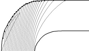
Particles of small size (10 microns) monitor the gaseous phase line current and the walls of virtually interacting. Larger particles 100 microns in diameter collide with the pipe wall after bending.

Large particles (300 and 500mkm) have a more direct path to the bending portion of the tube and collide with the wall with a high intensity. Low speed 300 micron particles can be trapped vortex gas flow and to be in it for a while. Large particles with a diameter of 500 mm, almost all come through the vortex. Only particles from the wall region with a very low speed to make a whirlwind return movement.

Fig. 2Curved orthogonal net curved pipe

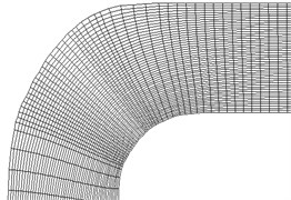
Fig. 3The velocity field in the curved section of the pipe

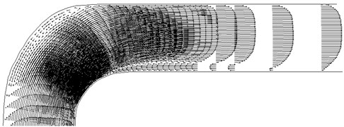
Fig. 4The particle trajectories diameter 10 mm

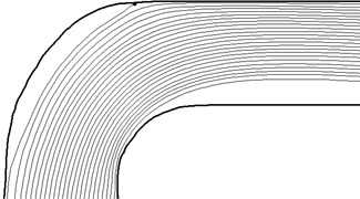
Fig. 5The particle trajectories a diameter of 100 microns

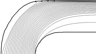
Fig. 6The particle trajectories diameter of 300 microns

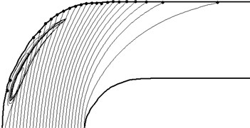
Fig. 7The particle trajectories diameter of 500 microns

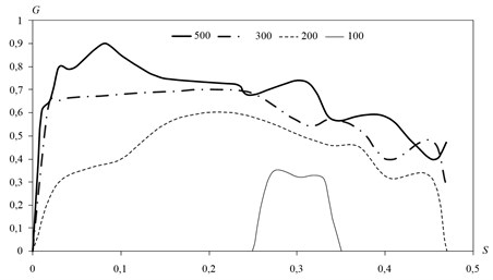
As a result of solving the problem of the motion of a two-phase mixture of particles and gas through the curved portion of the pipe calculated mass flows falling on the wall of particles of different sizes. The results are shown in Fig. 8.

Fig. 8 shows the distribution of massive flows of precipitating particles $G$ in several sizes. Coordinate $S$ measured at the tube wall. Mass flow rate $G$ is related to the mass flow rate of particles on a straight section of pipe (${\rho }_s{W}_s$). These data can be used to assess mechanical impact on the particles pipeline wall at different degrees of drying of natural gas.

Narrowing the flow cross section can be various kinds of control and measurement devices. The computational domain and the difference curvilinear grid shown in Fig. 9.

Fig. 8Distribution of mass flows deposited on particles of the wall of the pipe

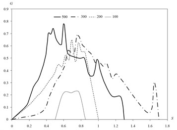
Fig. 9The difference in net contraction

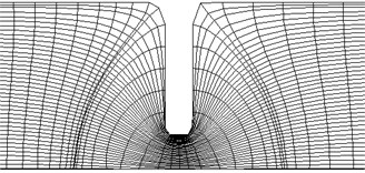
Fig. 10The flow field in the constriction

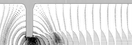
Fig. 11The particle trajectories diameter 10 mm

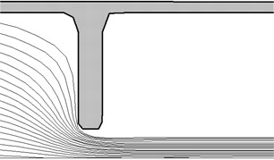
Fig. 12The particle trajectories diameter of 500 microns

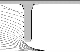
Fig. 13Mass flow deposited particulate

Calculation of the gas phase of motion parameters. The results are illustrated in Fig. 10.

Before narrowing of the pipe cross-section is observed stagnation zone with poor circulation flow in the wall region. After opening for jet nature is the presence of extensive areas (up to several pipe diameters) of the reverse flow. The movement of the condensed particles is shown in Fig. 11 and 12.

Small particles in this device follow the gas and do not fall into an obstacle.

Coarse particles have an intense effect on the structural member. precipitation intensity distribution for frequent diameter of 100-500 microns is shown in Fig. 13.

Here, the coordinate of $S$ corresponds to a distance from the pipe wall. Particles larger than 100 microns fall almost entire surface with obstacles fairly high intensity.

5. Conclusions

Figs. 6-8 demonstrate the possibility of increased erosion ash pipelines in areas of bending and rotation. The calculation of particle trajectories in the technological equipment of various kinds of shows at the option of either abrasive wear parts located in a stream, or an intense build-up and accumulation of hydrates.

The calculated results can be applied in the analysis of impact of solid particles of various sizes on the elements of gas pipelines.

References

-
Strizhov I. N., Hodanovich I. E. Gas Production. Institute of Computer Science, Moscow-Izhevsk, 2003, p. 376, (in Russian).
Oran Je., Boris Dzh. Numerical Simulation of Reacting Flows. Second Edition Cambridge University Press, 2001, p. 640.
Sekundov A. N. The use of differential equations for the turbulent viscosity and analysis of non-self plane currents. Bulletin of the Academy of Sciences USSR, Vol. 5, 1971, p. 114-127, (in Russian).
Gromadka II T., Lej Ch The Complex Boundary Element Method in Applied Sciences. Mir, Moscow, 1990, p. 303, (in Russian).
Benderskij B. Ja, Tenenev V. A. Experimental and numerical study of flows in axisymmetric channels of complex shape with blowing. Bulletin of the Russian Academy of Sciences, Vol. 2, 2001, p. 24-28, (in Russian).
Patankar S. Numerical Methods for Solving Problems of Heat Transfer and Fluid Dynamics. Jenergoizdat, Moscow, 1984, p. 150, (in Russian).
Benderskij B. Ja, Tenenev V. A. Spatial subsonic flows in areas with complex geometry. Math Modeling, Vol. 13, Issue 8, 2001, p. 35-39, (in Russian).
Amimul Ahsan Two Phase Flow, Phase Change and Numerical Modeling. InTech, 2011, p. 596.
About this article