Diacoptical analysis algorithms of topological site models of information backup and storage carrier

1. Topological models of tape transportation mechanism (TTM)

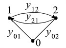
When considering the longitudinal vibrations in the tape path, the tape transportation mechanism [2] assumed that the portion of the tape is represented by two-node rod finite elements (Fig. 1). Sampling ribbon cable is provided so that finite elements nodes coincide with the fixed supports and lumped tape transportation mechanism. Fig. 2 and 3 shows the graph of two-node finite elements and a finite graph model of a tape portion.

Fig. 1Two-node rod finite elements

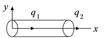
Fig. 2Directed graph two-node finite elements

Matrix stiffness, mass and damping finite elements have the form:

where $h_0$ – specific damping coefficient; $\rho$ – density of tape material; $\gamma$ – proportionality factor.

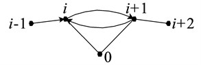
When preparing a formalized description of the graph finite elements model, the tape section is broken by directed graph on unimodal part as shown in Fig. 3. Fig. 4 shows a single-humped portion of the graph ${\gamma }_i$ – for the $i$-th vertex, which contains only the edges, entering the $i$-th vertex. Obviously, all unimodal parts of the graph, except in extreme, have the same structure, which is described by using the vertex sets as follows: ${\tau }_i=\left\{0,i-1,i+1\right\}$.

A set of weights of edges for the $i$-th vertex: $Y_i=\left\{y_{0i},y_{i-1,i},y_{i+1,i}\right\}$.

Fig. 3Directed graph finite elements model of section tape for two-node finite elements

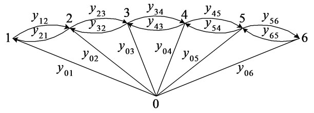
Fig. 4Unimodal part of graph γi

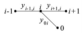
Fig. 6Graph of cubic finite elements

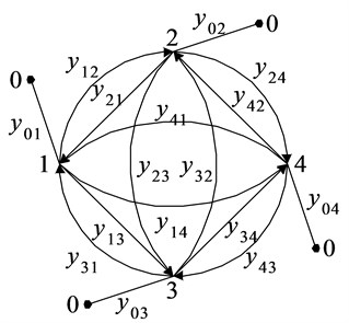
Fig. 5Part of graph γi,i+1

Weight functions of edges are defined by elements of matrixes of masses, stiffness and damping:

Since characteristic polynomial unimodal part ${\gamma }_i$ is obtained by adding the weights of the edges of the set $Y_i$, then it follows that they are equal to each other. As variable parameters, you can use the characteristics of finite elements $m_0$, $E$, $S$, $h_0$, $\rho$, $\gamma$ or some of them. It is also possible, knowing the dependence of the properties of the interested tape parameter of the designer, such as tension belts, to express a parametric function of edges via this parameter.

2. Algorithm for obtaining characteristic polynomial

The preparation of characteristic polynomial subgraph consisting of $n$ unimodal parts ${\gamma }_i$ is produced according to the formula:

where $\otimes$ is a sign of multiplying the characteristic polynomial special rules.

Consider the multiplication of two parts of the characteristic polynomial finite element graph ${\gamma }_i$ and ${\gamma }_{i+1}$. It can be shown that the set of tuples KOR2 for part ${\gamma }_{i,i+1}$ (fig. 5) consists of six tuples. Indeed:

Many tuples $KOR1$ are obtained by combining elements of vertex sets ${\tau }_i$ and ${\tau }_{i+1}$. Using conversion rules tuples and isolation circuits, we obtain a set of tuples ${\gamma }_{i,i+1}$:

The conversion process and tuples corresponding table $TU1$ multiplication are shown in Tables 1 and 2.

For any portion of the graph ${\gamma }_{i,i+1,\dots ,i+j}$, unimodal joining part formed ${\gamma }_{i+j}$ of the graph to ${\gamma }_{i,i+1,\dots ,i+j-1}$:

The induction method can prove that the set of tuples ${\gamma }_{i,i+1,\dots ,i+j}$ also has six tuples:

Thus, at each stage, the multiplication of characteristic polynomial of sets of tuples $KOR2$ is identical. Table multiplication tuples $TU2$ are also constant and are presented in Table 3.

Based on the above, a fast algorithm for obtaining partial characteristic polynomial finite element topology model is proposed for the two-node portion of the tape core finite elements.

Step 1. Set the number $N$ of finite elements section of tape.

Step 2. Calculate the number $n=N-1$ of unimodal parts subgraph containing all the vertices except the final one.

Step 3. We introduce the set $U=\left(U_1,U_2,\dots ,U_R\right)$ of variable parameters of finite elements.

Step 4. Construct parametric function of edges unimodal parts ${\gamma }_i$ in a finite element model.

Step 5. Form the characteristic polynomial part of $H\left({\gamma }_i\right)$ unimodal parts ${\gamma }_i$ in an ordered set of terms $SL\left({\gamma }_i\right)$ and a set of numbers $M\left({\gamma }_i\right)$, defining elements of vertex sets ${\tau }_i$, of appropriate term characteristic polynomial.

Step 6. $i$ = 2.

Step 7. Form the characteristic polynomial portion $H\left({\gamma }_{i,i+1}\right)=H\left({\gamma }_i\right)\otimes H\left({\gamma }_{i+1}\right)$ for a plurality of numbers of tuples $MKOR\left({\gamma }_{i,i+1}\right)$ and a plurality of $SL\left({\gamma }_{i,i+1}\right)$ using the multiplication table (Table 2).

Step 8. $j$ = 2.

Step 9. Form the characteristic polynomial portion ${\gamma }_{i,i+1,\dots ,i+j}$ according to the formula

For a set of terms $SL\left({\gamma }_{i,i+1,...,i+j}\right)$ and a set of corresponding numbers of tuples $MKOR\left({\gamma }_{i,i+1,...,i+j}\right)$ using multiplication tables tuples $TU2$(table 3).

Step 10. $j$ = $j$+1.

Step 11. If $j$ = $n$ – 1, then go to step 9 otherwise to step 12.

Step 12. The work end.

Increased performance of the algorithm is carried out by: identity unimodal parts as input formalized description and the formation of characteristic polynomial unimodal parts ${\gamma }_i$ done once; lack of stage definition $w_1$ and $KOR2$ after multiplication of partial characteristic polynomial; there is no need to form the multiplication tables at each stage of the multiplication of characteristic polynomial.

3. TTM topological model in study of flexural vibrations portions of tape

When considering the flexural vibrations of the tape portion is represented by cubic core finite elements with two internal nodes. Elastic bending line in this case is described by a polynomial of the third degree. Matrixes of masses and stiffness of the cubic finite elements have dimension 4×4.

Fig. 7Graph of finite elements model of tape section using cubic finite elements

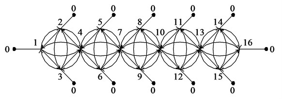
Fig. 8Graph of three vertices of finite elements model for cubic finite elements

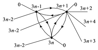
Fig. 9Graph of unimodal parts γ1

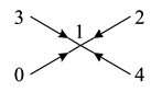
Fig. 10Graph of unimodal parts γN

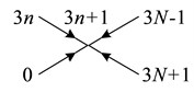
Fig. 11Graph of unimodal parts γ3n-1

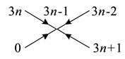
Fig. 12Graph of unimodal parts γ3n

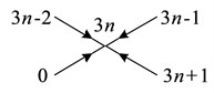
Fig. 13Graph of unimodal parts γ3n+1

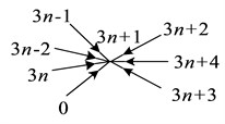
Fig. 6 is a graph of the cubic finite elements, and Fig. 7 shows a graph of the finite-element model of tape section, consisting of a few cubic finite elements. Divide the graph into parts, cutting the arcs of the graph lines $0A_j$, as shown in Fig. 7. It is easy to note that the graph represents the connection of three vertex parts of the same structure shown in Fig. 8, except for the final part of the graph. Unimodal part of the graph to the end vertices are shown in Fig. 9 and 10. The characteristic polynomial graph finite elements model can be obtained by multiplying its parts to characteristic polynomial by the formula:

where $N$ – number of finite elements, $n$ – serial number of finite element.

In turn, the three-vertex graph ${\gamma }_{3n-\mathrm{1,3}n,3n+1}$ divided by unimodal part of ${\gamma }_{3n-1}$, ${\gamma }_{3n-1}$, ${\gamma }_{3n+1}$ shown in Figs. 11-13. Vertices of the set of parts are respectively:

Sets of weights of the edges unimodal parts are equal:

where $y_{\mathrm{0,3}n-1}=m_{22}{p}^2+c_{22}$, $y_{3n-\mathrm{1,3}n}=m_{23}{p}^2+c_{23}$, $y_{3n+\mathrm{2,3}n+1}=m_{21}{p}^2+c_{21}$, $y_{3n-\mathrm{2,3}n-1}=m_{12}{p}^2+c_{12}$, $y_{3n+\mathrm{1,3}n}=m_{43}{p}^2+c_{43}$, $y_{3n+\mathrm{3,3}n+1}=m_{31}{p}^2+c_{31}$, $y_{3n,3n-1}=m_{32}{p}^2+c_{32}$, $y_{\mathrm{0,3}n+1}=m_{44}{p}^2+c_{44}$, $y_{3n+\mathrm{4,3}n+1}=m_{41}{p}^2+c_{41}$, $y_{3n+\mathrm{1,3}n-1}=m_{42}{p}^2+c_{42}$, $y_{3n-\mathrm{2,3}n-1}=m_{14}{p}^2+c_{14}$, $y_{\mathrm{0,3}n}=m_{33}{p}^2+c_{33};y_{3n-\mathrm{1,3}n+1}=m_{24}{p}^2+c_{24}$, $y_{3n-\mathrm{2,3}n}=m_{13}{p}^2+c_{13}$, $y_{3n,3n+1}=m_{34}{p}^2+c_{34}$.

Partial characteristic polynomials three-vertex parts are obtained by multiplying the characteristic polynomial unimodal parts.

Multiplication by the formulas (9) and (12) makes it possible to develop an effective algorithm for obtaining the characteristic polynomial of the finite element model for cubic finite elements.

When developing an algorithm, the following was considered:

1) the set of tuples $KOR2$, obtained by combining of parts ${\gamma }_{3n-1}$ and ${\gamma }_{3n}$, consists of 9 tuples, and the corresponding table multiplication $TU1$ (Table 4) is a constant for all three-vertex of parts;

2) the set of tuples $KOR2$, obtained by combining of parts ${\gamma }_{3n-1}$ and ${\gamma }_{3n}$, and the corresponding table multiplication $TU2$ (Table 5) is a constant, the number of tuples is equal to 35;

3) sets of $w_1$ and $w_2$, and three-vertex part of ${\gamma }_{3n-\mathrm{1,3}n,3n+1}$ are equal $w_1=\left\{3n-\mathrm{1,3}n,3n+1\right\}$, $w_2=\left\{3n-\mathrm{2,3}n+\mathrm{2,3}n+\mathrm{3,3}n+4\right\}$.

4) when multiplying the characteristic polynomial three-vertex parts $H\left({\gamma }_{3n-\mathrm{1,3}n,3n+1}\right)$, the formation process of tuples happens by special rules, except that a plurality of tuples formed by a combination of the sets of tuples $KOR2$ of these parts.

Similarly, it is possible to construct algorithms for other types of finite elements, taking into account the peculiarities of topological models of specific types of finite elements.

Also the algorithm of topological analysis of a dynamic model of the tape transport mechanism, is represented as a set of lumped masses [4] related to the tape portion, the example of the longitudinal tape vibrations, presenting it as a two-node areas rod finite elements.

These characteristic polynomial of the transfer function of the system and discrete-continuous model [5] is presented in the form of a plurality of predetermined functions of variable parameters $U=\left\{U_{KE},U_D\right\}$. With the expression of the characteristic polynomial and the transfer function of the system in alpha-numeric form, as a function of the actual parameters of the tape transport mechanism can obtain the frequency equation, the frequency characteristics of the tape transport mechanism – the amplitude-frequency characteristic, the logarithmic amplitude-frequency characteristic, the phase-frequency characteristic, spending optimal synthesis parameters of tape transport mechanism.

4. Conclusion

The synthesis method of tape transport mechanisms, including the identification of a dynamic model of the tape transportation mechanism, the construction of a topological model, formalized description and analysis of diacoptical models of the tape transport mechanism with lumped and distributed parameters, as well as the synthesis method of the tape transport mechanism parameters for the frequency spectrum were developed [1, 3].

An efficient algorithm diacoptical analysis, enabling you to get characteristic polynomial and PPS systems as function parameters for focused and undirected graphs, was provided.

It is the best way to describe the structure of the graph parts with a plurality of the internal connection of the vertices and the set of tuples consisting of external connecting vertices and zero vertex, allowing reducing the count description and simplifying the process of contours finding.

The concept of edges is introduced in the form of a multi-dimensional polynomial function of variable parameters, which gives a great opportunity in the choice of the designer’s investigated parameters of the system.

Fast algorithms for topological analysis of graphs of finite element models of the carrier sites for different types of finite elements are developed allowing for minimal time to obtain the transfer function of the system of a graph as a function of parameters finite elements.

The dynamic and topological model of the tape transportation mechanism is identified as a discrete-continuous system and an effective algorithm is proposed for obtaining characteristic polynomial and the system transfer function based on the diacoptical analysis allows taking into account the carrier distribution parameters.

References

-
Elkin V. S., Lyalinv E. Analysis of methods of spectral synthesis of conservative dynamical systems. VestnikISTU: Mathematical Modeling of Radio-Electronic Means of Telecommunication Systems, Izhevsk, 2002, p. 29-35, (in Russian).
Elkin V. S., Nistyuk A. I. Algorithms analysis of diacoptical topological models plots tape carrier-playback recording equipment VestnikISTU: Intelligent Information Technology in Telecommunications and Telemetry, Izhevsk, 2002, p. 34-38, (in Russian).
Elkin V. S., Nistyuk A. I. Methods and algorithms for synthesis of dynamic systems of frequency spectrum. VestnikISTU: Mathematical Modeling of Radio-Electronic Means of Telecommunication Systems, Izhevsk, 2002, p. 28-33, (in Russian).
Elkin V. S., Nistyuk A. I., Lyalin V. E. A formal description of algorithm and analysis diacoptical topological models of dynamic systems with lumped parameters. VestnikISTU: Mathematical Modeling of Radio-Electronic Means of Telecommunication Systems, Izhevsk, 2002, p. 35-42, (in Russian).
Elkin V. S. Formal description of algorithm and diacoptical analysis of discrete-continuous model of dynamic system information registrar. VestnikISTU: Mathematical Modeling of Radio-Electronic Means of Telecommunication Systems, Izhevsk, 2002, p. 43-44, (in Russian).
Chua L. O. Chen Li-Kuan Diacoptic and generalized hybrid analysis. IEEE Transactions on CAS, Vol. 23, Issue 12, 1976, p. 694-705.
About this article