Solutions of seepage equations in curvilinear coordinates

1. Introduction

In the case of complex shapes study area is desirable to use of computational grids borders, adapted to current conditions. The use of grids with rectangular border approximation leads to considerable complication of calculation algorithms to implement the boundary conditions.

2. Mathematical model

To build a grid on a curved surface, consider the geometry of a regular piece of the surface $S$ defined by the equation in three-dimensional Euclidean space:

where $u$, $v$ some arbitrary coordinates. The orthogonal grid on the surface given by the equations $\xi =\xi (u,v)=const$, $\eta =\eta (u,v)=const$. For orthogonal lines on the surface of the relation:

where $n$, $\tau$ – normal and tangent to the line.

Functions $\xi (u,v)$, $\eta (u,v)$ must satisfy the system of equations [6]:

which is a generalization of the Cauchy-Riemann conditions.

To solve the system (3) differentiate the first equation by $v$, second by $u$, and add on them. As a result, we obtain a second differential operator:

where $E(u,v)={\left(\frac{\partial x}{\partial u}\right)}^2+{\left(\frac{\partial y}{\partial u}\right)}^2+{\left(\frac{\partial z}{\partial u}\right)}^2$, $G(u,v)={\left(\frac{\partial x}{\partial v}\right)}^2+{\left(\frac{\partial y}{\partial v}\right)}^2+{\left(\frac{\partial z}{\partial v}\right)}^2$, $F(u,v)=\frac{\partial x}{\partial u}\frac{\partial x}{\partial v}+\frac{\partial y}{\partial u}\frac{\partial y}{\partial v}+\frac{\partial z}{\partial u}\frac{\partial z}{\partial v}$ – factors of fundamental quadratic form of the surface.

3. Algorithm and computational experiments

An algorithm for constructing orthogonal grid consists of consecutive solutions of the equation (4) and equation ${\nabla }^2\xi =0$ with the appropriate boundary conditions. For variable $\eta$ at one boundary set values $\eta =0$, on the other $\eta =1$, on the other borders $\frac{\partial \eta }{\partial n}=0$, where $n$ – normal to the boundary. From equation (2) are determined by the boundary conditions for the variable $\xi$ and the equation ${\nabla }^2\xi =0$ is solved. Equations (1) and $\xi =\xi (u,v)=const$, $\eta =\eta (u,v)=const$ define the position of the mesh nodes on the curved surface.

Equation (4) approximated the system of difference equations in the nine-pattern. The system of differential equations was solved by an iterative method of conjugate gradient regularization [1].

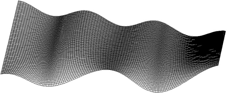
In the area shown in Fig. 1, a joint motion of the two phases: wetting and wetting liquids is considered. In this case, there are four unknown variables and hence four equations: two differential and two algebraic ones [2-4].

where $f=\left\{w,o\right\}$ – the index for the wetting and non-wetting phase; $S_f$ – saturation of the pore volume phase $f$; $P_c$ – capillary pressure. It is believed that there is between $S_f$ and $P_c$ the functional dependence ${\mathrm{\lambda }}_f\left(\mathbf{r}\right)={\mathbf{k}}_f\left(\mathbf{r}\right)/{\mu }_f$, ${\gamma }_f={\rho }_{f}g$, $\mathbf{r}\in \mathrm{\Omega }\subset {\stackrel{-}{\mathrm{\Omega }}}^3$; $P_f\left(\mathbf{r}\right)$ – pressure at the point $\mathbf{r}\in \mathrm{\Omega }$; $\stackrel{-}{\mathrm{\Omega }}$ – filtering domain with boundary $\mathrm{\Gamma }$; $\mathbf{n}$ – outward normal; ${\mathbf{k}}_f$ – diagonal tensor absolute permeability; $h$ – seam thickness; $Z$ – depth; ${\mu }_f$ – liquid viscosity; $\rho {}_f{}^{\mathrm{}}\mathrm{}$ – liquid density; $g$ – acceleration of gravity; $Q_f$ – power sources; $\phi \left(\mathbf{r}\right)=\phi °\left(\mathbf{r}\right)\left(1+c_{\phi }\left(P-P°\right)\right)$ ; $\phi \left(\mathbf{r}\right)$ – porosity; $B_f$ - volumetric coefficient; $P$ – characteristic pressure.

Fig. 1Difference grid on curved surface

In curvilinear orthogonal coordinates $(\xi ,\eta )$, the divergence of the gradient operator is as follows:

where $e={\left(\frac{\partial x}{\partial \eta }\right)}^2+{\left(\frac{\partial y}{\partial \eta }\right)}^2+{\left(\frac{\partial z}{\partial \eta }\right)}^2$, $g={\left(\frac{\partial x}{\partial \xi }\right)}^2+{\left(\frac{\partial y}{\partial \xi }\right)}^2+{\left(\frac{\partial z}{\partial \xi }\right)}^2$, $w=\sqrt{eg}$.

Then the difference approximation of two-dimensional filtering equation difference is a five-point pattern as in the Cartesian coordinates. The difference in rates is the difference in accounting factors $\frac{1}{w}$, $\frac{e}{w}$, $\frac{g}{w}$. Difference boundary conditions maintain their appearance. Therefore, the entire numerical algorithm, which is implemented into the Cartesian coordinates, is fully maintained.

Fig. 2Isolines S=const

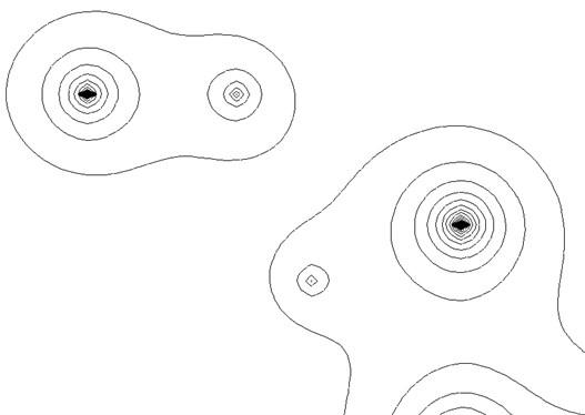
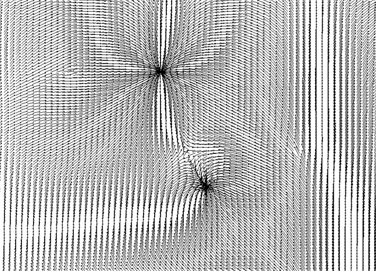
In the following figures, the results of calculations for the reservoir, which has a curved shape, as in Figure 1 are shown. There is a problem of two-phase filtration. When $t=3.2$ contour lines $S=const$ are shown (Figure 2), as well as the movement of water (Figure 3) and oil (Figure 4).

Fig. 3Water flow

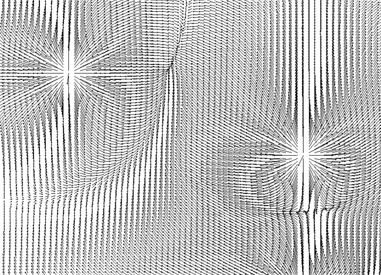
Fig. 6Oil flow

4. Conclusions

The developed approach to the construction of the difference of the orthogonal curvilinear grid allows the calculation of filtration processes in formations with complex geometry. Accounting reservoir capacity with a relatively small thickness allows solving problems in a quasi-three-dimensional setting.

References

-
Golub J., Van Loan Charles Matrix Computations (3rd Edition). Johns Hopkins University Press, Baltimore, MD, USA, 1996, p. 728.
Aziz H., Settarov E. Mathematical Modeling of Reservoir Systems. Institute of Computer Science, Moscow-Izhevsk, 2004, p. 416. Original Publication: “Nedra”, Moscow, 1982, (in Russian).
Chanson, H. Applied Hydrodynamics: An Introduction to Ideal and Real Fluid Flows. CRC Press, Taylor and Francis Group, Leiden, The Netherlands, 2009, p. 478.
Economides Michael J., Nolte Kenneth G. Reservoir Stimulation. Wiley, USA, 2000, p. 856.
About this article