An improved component mode synthesis method for interval uncertainty analysis

1. Introduction

During the last decades, the FEM has been applied widely in the dynamic analysis of the deterministic models. But every manufacturing process naturally introduces some product variability, which is inevitable, such as manufacturing tolerances, material deviation, and so on. And the presence of uncertainties can affect significantly the dynamical behavior of the model. Therefore, a deterministic model is not sufficient to analyze structure dynamics. What's more, due to the growing demands imposed on new products the influence of all relevant uncertainties in properties has begun to be paid more and more attention in the static and/or dynamic analysis of structures.

According to previous works, one can distinguish probabilistic and non-probabilistic approaches as two main categories. The non-probabilistic approach is retained in this paper. In non-probabilistic approaches, the interval methods are based upon the interval concept for the presentation of uncertainty model properties, and so far, has been reported in some literatures [1, 2].

With the development of industry technology, a very large number of degrees of freedom are usually required for complex FE model. The calculation cost of the interval finite element method can be prohibitively expensive. Component mode synthesis (CMS) technique is a favored solution method, which can significantly reduce the model size. CMS was introduced firstly in the 1960s by Hurty [3], which focused on undamped linear vibration system. In following decades，CMS methods have been extensively developed [4-6]. Moreover, CMS currently plays an important role in the dynamic analysis of the sophisticated structures. In Ref. [7, 8], the fixed interface CMS methods was employed to analysis of the elastic multibody systems, it was shown that the numerical costs can be reduced efficiently. He Huan et al. [9] proposed a hybrid coordinates CMS approach for a localized nonlinear system. Kawamura and Naito [10] presented a method for the analysis of nonlinear forced vibration of a multi-degree-of-freedom system. As a result, it was shown that the approach proposed in this paper is effective in the case with rigid modes in components. Klaus-Jürgen Bathe and Jian Dong [11] utilized subspace iteration method to improve the component mode synthesis solutions. Zhe Ding et al. [12] presented a free interface CMS method for viscoelastic ally damped systems. In this paper, two residual attachment modes of viscoelastic ally damped systems are proposed to reduce the mode truncation error. Two new CMS methods were proposed in Ref. [13] for generally damped systems. In order to reduce the time consumption in re-analyses of large-order models, Costas Papadimitriou [14] applied Craig-Bampton CMS method to finite element model updating.

In general, the individual components are analyzed individually and subsequently they are assembled to produce a reduced model of the whole structure. The benefits concerning the quantification and propagation of uncertainty arise from that fact that each component can be treated independently. When one or more components involve uncertainties in properties, only the components which are uncertain need to be reanalyzed. Furthermore, the uncertain data can be naturally introduced at the component level. Quang Hung Tran et al. [15] proposed an alternative CMS method for damped vibroacoustic problems. In this paper, the robust bases were constructed to solve the problem of uncertainties propagation. The results show that the proposed method results in significant time reduction. D. Sarsri et al. [16] utilized the CMS method to reduce the size of large FE systems with linear and nonlinear stochastic parameters, and they investigated the frequency transfer functions of the stochastic systems. Hilde De Gersem et al. [17] combined the CMS method with the interval and fuzzy finite element method to analyze the eigenvalue and frequency response function of structures with uncertain parameters. L. Hinke et al. [18] applied the fixed-interface CMS method to the analysis of structures with uncertainty. In this paper, Quantification and propagation of uncertainty in properties was discussed. S. A. Chentouf et al. [19] proposed a hybrid method for modelling parametric and non-parametric uncertainties. Craig-Bampton CMS method was adapted to approximate reanalysis process. Oliviero Giannini and Michael Hanss [20] proposed a component mode transformation method, which couples the capabilities of the standard transformation with the computational advantages of the CMS approach, for mechanical systems with uncertain parameters.

Above methods which apply the constraint interface CMS to the analysis of structures with non-deterministic properties can reduce efficiently the time consuming. The realistic quantification of the non-deterministic behavior of components is usually obtained through experiments, and then the uncertainties of the components in properties can be propagated to the whole system. Nevertheless, the major limitation of the methods utilizing constraint modes is the inability to easily obtain the experiment data. An improved free interface CMS combined with interval methods was proposed in order to reduce the computation time of interval dynamic analyses. In this paper, the whole dynamic system is separated into several substructures, and only these substructures which involve non-deterministic properties are analyzed by the small parameter perturbation method. The synthesis equations can be deduced by assembling all of the equations of components in terms of the interface compatibility conditions. The interval dynamic analysis of a bridge structure is given to illustrate the application of the method proposed in this paper and a Monte Carlo simulation is then used as a reference. Modal tests have been conducted to the structure with different combination of pieces, comparison between experimental results and the analytical results are also given to demonstrate the validation of the presented method.

2. Perturbation analysis of components with parametric uncertainties

In general, the system can be divided into several components. The undamped vibration equation of the motion of arbitrary components can be expressed as:

where $\mathbf{{\rm M}}$ and $\mathbf{K}\in {\mathbb{R}}^{n\times n}$ are the mass and stiffness matrices of the component, respectively. $\mathbf{u}$ and $\mathbf{f}\in {\mathbb{R}}^{n\times 1}$ are, respectively, the generalized displacement and external force vectors. $n$ is the DOF of the component. Denote ${\mathrm{\Phi }}^l\in {\mathbb{R}}^{n\times l}$ as the first $l$ order normal modes retained, which can be obtained by solving the eigenvalue problem.

According to interval finite element method the uncertain structural parameters can be written into $a=\left[\begin{array}{ll}\underset{\_}{a}& \stackrel{-}{a}\end{array}\right]$. Where $\underset{\_}{a}$ and $\stackrel{-}{a}$ are, respectively, the infimum and supremum of variables.

$a$ can be also written in the perturbed formulation:

where $\delta a=a^c{e}_{\mathrm{\Delta }}$, $a^c=\frac{1}{2}\left(\overline{a}+\underset{\_}{a}\right)$, $∆a=\frac{1}{2}\left(\overline{a}-\underset{\_}{a}\right)$, $e_{∆}\in [-1.1]$.

With the variables perturbation, the mass matrices, stiffness matrices, eigenvalues and eigenvectors of the component according to Eq. (2) can be expressed as follows:

Assume that there exists a matrix $\mathbf{\varphi }\in {\mathbb{R}}^{n\times (n-l)}$ can be expressed as:

where $\mathbf{w}$ is a matrix to be solved and $\tilde{\mathbf{\varphi }}$ is composed of $n-l$ linear independent vectors which can be written as:

We consider the weighted-orthogonal relationship:

Substituting Eq. (4) into Eq. (6) will give:

Eq. (7) can be also written as:

Substitution of Eq. (8) into Eq. (5) will lead to:

We consider that the retained lower order mode matrix ${\mathrm{\Phi }}^l$ is normalized with respect to mass matrix, Eq. (9) can be simplified as:

Substitution of Eq. (3) into Eq. (10) and then neglect the higher-order terms will give:

It is not difficult to prove that ${{\mathrm{\Phi }}^l}^{{\rm T}}\mathbf{K}\varphi =0$.

We can define the equivalent full modes matrix as $\mathrm{\Phi }=\left[\begin{array}{ll}{\mathrm{\Phi }}^l& \mathbf{\varphi }\end{array}\right]=\left[\begin{array}{ll}{\mathrm{\Phi }}^{lc}+\delta {\mathrm{\Phi }}^l& {\mathbf{\varphi }}^c+\delta \mathbf{\varphi }\end{array}\right]$, and the physical coordination of the component can be written by:

where:

By splitting $\mathbf{\beta }$ between ${\beta }_l$ and ${\beta }_h$ according to the retained lower-order modes and higher-order modes, where subscripts $l$ and $h$ denote the number of retained lower-order modes and higher-order modes to be respectively reduced, we can rewrite Eq. (12) as:

Substitution of Eq. (14) into Eq. (1) and pre-multiplication of the resulting equation by ${\mathrm{\Phi }}^T$ will give:

Denote:

The second line of Eq. (15) can be written as:

By Laplace transformation of above equation can give:

Retaining only the first item of the Taylor expansion of Eq. (19), and the inverse Laplace transform on the resulting equation lead to:

Substituting Eq. (20) into Eq. (14) will give:

where $\mathbf{G}\in {\mathbb{R}}^{n\times n}$ is the residual flexibility attachment matrix and can be written in the following form as:

The stiffness matrix of the system is singular when there are rigid modes in the component, so the residual flexibility attachment matrix cannot be acquired by inversing the stiffness matrix directly. Quite different from the previous papers, the residual flexibility matrix presented in this paper can be obtained by computing the inverse of equivalent higher order stiffness matrix ${\mathbf{K}}_h$ instead of $\mathbf{K}$. And since the equivalent higher order stiffness matrix ${\mathbf{K}}_h$, which is just related to the equivalent higher modes, is a nonsingular matrix, it is easier to calculate the residual flexibility matrix by Eq. (22).

Substitution of Eq. (11) into Eq. (17), we can acquire the perturbation expression ${\mathbf{K}}_h$, and one order approximation for the matrix inversion of ${\mathbf{K}}_h$ can be expressed as:

In the same way, we can acquire:

where:

The physical DOFs can be portioned into a set of interior DOFs ${\mathbf{u}}_i$ and a set of interface DOFs ${\mathbf{u}}_j$. Eq. (12) can be rewritten in the form:

where ${\mathbf{f}}_j$ is the force vector at the junctions and ${\mathbf{f}}_i$ is external force vector.

The interface displacement ${\mathbf{u}}_j$ can be expressed by partition of Eq. (27):

3. Components synthesis equations

For convenience, consider the synthesis of components $a$ and $b$. According to Eq. (28) the displacement of interface of the two components can be written as:

The physical displacement continuity and force continuity at the conjunction region are employed to assemble the components. These conditions can be expressed as follows:

Substituting Eq. (29) an Eq. (30) into Eq. (31), and Eq. (32) is introduced together to give:

where:

Substitution of Eq. (24) into Eq. (34) will lead to:

where:

According to Eq. (33), we can obtain:

Don’t consider the external force, substituting Eq. (33) into Eq. (38) and Eq. (39) will give:

where:

We can also rewrite Eq. (40) as:

4. Interval eigenvalue analysis of synthesis model

The first order perturbation item of the eigenvalues of the reduced model can be expressed as:

where ${\stackrel{-}{\lambda }}_i$ and ${\stackrel{-}{\mathrm{\Phi }}}_i$ are the eigenvalues and the eigenvectors of the reduced model, respectively, which are obtained from the deterministic model.

We consider that the mode matrix $\stackrel{-}{\mathrm{\Phi }}$ is normalized with respect to mass matrix $\stackrel{-}{\mathbf{M}}$, denote $\delta \stackrel{-}{\mathbf{K}}$ and $\delta \stackrel{-}{\mathbf{M}}$ as $\sum _{j=1}^r\frac{\partial \stackrel{-}{\mathbf{K}}}{\partial {\alpha }_j}\cdot \delta {\alpha }_j$ and $\sum _{j=1}^r\frac{\partial \stackrel{-}{\mathbf{M}}}{\partial {\alpha }_j}\cdot \delta {\alpha }_j$, the interval function of $\delta {\lambda }_i$ can be written as:

The interval of $\delta \stackrel{-}{\lambda }$, $\delta \stackrel{-}{\lambda }/{\stackrel{-}{\lambda }}^c$ can be obtained via interval method, then according to Eq. (50) we can acquire the interval of the eigenvalues of the system and the influencing degree of the non-deterministic factor to the natural frequencies.

5. Examples

5.1. Numerical example

5.1.1. Model description

For demonstration purposes, a bridge is considered. The length of the bridge is 108 m, the width of it is 11.2 m. As shown as in Fig. 2 and Fig. 3, the bridge is separated into two physical components. The component $a$ contains 126 two-node beam elements, 50 nodes each has 6 DOFs, 300 DOFs in total. The component $b$ has 111 two-node beam elements, 40 nodes each has 6 DOFs, 240 DOFs in total. The beam element is circular hollow in cross-section. And the Parameters used in the model of the bridge are listed in Table 1.

Fig. 1The bridge structure

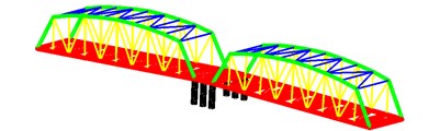
Fig. 2The component a

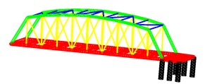
Fig. 3The component b

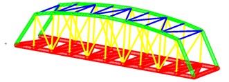
Table 1Parameters used in the model of the bridge

Young’s modulus / GPa	210
Poisson ratio	0.3
Density / kg/m3	7800
Internal diameter/external diameter of the red group / m	0.88/1.04
Internal diameter/external diameter of the green group / m	0.76/0.8
Internal diameter/external diameter of the yellow group / m	0.28/0.32
Internal diameter/external diameter of the blue group / m	0.26/0.30
Internal diameter/external diameter of the black group / m	1.2/1.4

5.1.2. Natural frequency analysis of deterministic model

The natural frequencies are calculated using the proposed synthesis method, and compared with those obtained using the full FE model in Table 2, where $l$ indicates the number of the lower retained modes of each component to formulate the synthesis equations (See Eq. (48)).

Table 2Comparison of the eigenvalues from the presented method and the full FEM (Unit: Hz)

Mode order	$l=$ 10	$l=$ 15	$l=$ 20	$l=$ 25	Full FEM
1	2.8798	2.8797	2.8797	2.8797	2.8717
2	2.8899	2.8898	2.8898	2.8898	2.8818
3	5.1982	5.1954	5.1953	5.1950	5.1936
4	5.2580	5.2513	5.2511	5.2507	5.2491
5	6.0000	5.9975	5.9961	5.9960	5.9945
6	6.0274	6.0223	6.0200	6.0198	6.0182
7	7.9113	7.9092	7.9065	7.9061	7.9039
8	7.9826	7.9813	7.9801	7.9799	7.9778
9	8.9783	8.9578	8.9319	8.9286	8.9261
10	9.6052	9.5749	9.5468	9.5449	9.5429
11	10.2119	10.2026	10.2020	10.2006	10.198
12	10.3199	10.2419	10.2410	10.2391	10.237

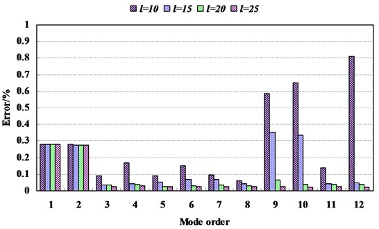
We can define the error measure for the natural frequency as $\epsilon =\left|{\omega }_s-{\omega }_f\right|/\left|{\omega }_f\right|\times$ 100 %, where ${\omega }_s$ refer to the natural frequency acquired from the synthesis model, and ${\omega }_f$ refer to the natural frequency acquired from the full FE model. The comparison of error measure for natural frequencies is shown in Fig. 4. It is observed that the errors reduce for higher modes and the maximum error is less than 0.3 % when more than 20 modes are comprised in the synthesis model.

Fig. 4Comparison of error measure for natural frequencies

The CPU time of natural frequency analysis spent on the reduced model and the full FE model is listed in Table 3. The CPU time ratio is defined by $t_s/t_f\times$100 %, where $t_s$ is the CPU time spent on the reduced model, $t_f$ is the CPU time spent on the full model. Obviously, it can significantly increase the calculation efficiency by using the CMS method presented in this paper.

Table 3Comparison of the CPU time spent on the synthesis models and full FE model

	Synthesis models				Full FE model
	$l=$ 10	$l=$ 15	$l=$ 20	$l=$ 25
CPU time / s	20.2	44.6	52.6	69.7	2247.0
CPU time ratio	0.9 %	2.0 %	2.3 %	3.1 %

5.1.3. Interval eigenvalue analysis

We consider that Young’s Modulus of component $a$ and $b$ is modeled by an interval quantity which can be expressed as:

$E_i^I=\left[E^c-\beta E^c,E^c+\beta E^c\right],i=a,b,$

where $E^c=$ 210 GPa, $\beta =$ 5 %.

Monte Carlo method is widely used to predict the response of the systems with significant uncertainties or the system exhibited probabilistic characteristics. It is well known that the accuracy of the Monte Carlo approach is dominated by the number of samples of the uncertainties. The Larger number of the samples always means the higher accuracy of the result obtained by using the Monte Carlo method. However, with the increasing number of samples, the computational costs become expensive and extremely time consuming, especially for the dynamic analysis of the complex FE model with numerous number of DOFs. Since the Monte Carlo method can lead to highly accurate result for predicting response of the system with uncertainties, we take the results obtained from the Monte Carlo approach as the standard values to evaluate the accuracy of the results obtained by using the proposed method. The intervals of natural frequencies obtained from the method proposed in this paper and those obtained from Monte Carlo method with 100 runs due to an uncertainty on the Young’s modulus are listed in Table. 4. It shows that the synthesis method gives very close bounds to the Monte Carlo method.

Table 4Intervals obtained from presented method and Monte Carlo method when β= 5 %

Mode order	The presented method	The Monte Carlo method
1	[2.8060, 2.9534]	[2.8138, 2.9436]
2	[2.8154, 2.9642]	[2.8226, 2.9540]
3	[5.0613, 5.3279]	[5.0698, 5.3214]
4	[5.1175, 5.3827]	[5.1229, 5.3783]
5	[5.8425, 6.1481]	[5.8493, 6.1423]
6	[5.8672, 6.1706]	[5.8713, 6.1665]
7	[7.7026, 8.1072]	[7.7142, 8.0976]
8	[7.7758, 8.1824]	[7.7898, 8.1744]
9	[8.6856, 9.1612]	[8.7001, 9.1467]
10	[9.2806, 9.7976]	[9.2986, 9.7736]
11	[9.9374, 10.4592]	[9.9462, 10.4504]
12	[9.9688, 10.5042]	[9.9833, 10.4897]

Fig. 5The envelopes of change rate of natural frequencies when β= 5 %

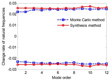
The change rate of natural frequencies can be defined as $\stackrel{-}{\epsilon }=\frac{\stackrel{-}{\omega }-{\omega }_c}{{\omega }_c}\times$100 % and $\underset{\_}{\epsilon }=\frac{\underset{\_}{\omega }-{\omega }_c}{{\omega }_c}\times$100 %, where ${\omega }_c$ is the natural frequency obtained from the deterministic model, $\stackrel{-}{\omega }$ and $\underset{\_}{\omega }$ are, respectively, the upper and lower bounds correspond to the natural frequency. As shown as in Fig. 5, the upper and lower change rate bound computed by CMS gives a narrow envelop of the results using Monte Carlo method. The reduced model induces hardly any loss of accuracy as the interval results of Monte Carlo method. In addition, it needs to take around 100 minutes by using the Monte Carlo method, while it just needs to take around 2 minutes by using the synthesis method. Obviously, the method presented in this paper can greatly reduce the time consumption.

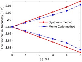
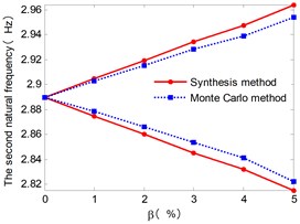
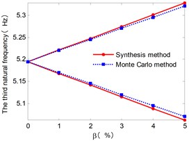
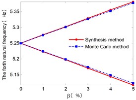
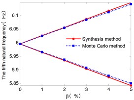
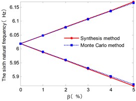
Fig. 6 shows the envelopes of the first six natural frequencies for the case with different $\beta$. The natural frequency intervals increase with the increase of $\beta$. And the upper and lower bound obtained from the approach presented in this paper also gives a narrow envelop of the Monte Carlo results.

Fig. 6The envelopes of lower six natural frequencies with increasing of β

a)

b)

c)

d)

e)

f)

5.2. Experiment demonstration

The bolted plate is a kind of typical connecting structure, whose dynamics characteristics is generally influenced significantly by the uncertainties of material and connection stiffness. Two plates and two bolts are randomly selected from the test pieces shown in the Fig. 7 and the setup for modal testing of the connecting structure is shown in Fig. 8.

Fig. 7Photograph of test pieces

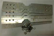
Fig. 8Photograph of modal testing system

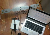
Fig. 9(a) shows the FE model of the bolted plates. As shown as in the Fig. 9(b) and Fig. 9(c), the connection structure is separated into component $a$ and component $b$, and they are connected by using two bolts. The plates are modeled by shell elements. The bolts which are the connection between substructure $a$ and $b$ are modeled by beam elements.

The diameter of each bolt and the Young’s modulus of each plate are determined in advance. The interval of the diameters of those bolts is [5.94 mm, 6.04 mm], while the interval of the Young’s modulus of those plates is [66.2 GPa, 70.3 GPa].

Fig. 9FE model of bolted plate and components a and b

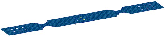
a) FE model of bolted plate

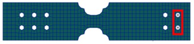
b) Component $a$

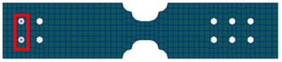
c) Component $b$

Table 5Intervals obtained from the synthesis models and experimental model (Unit: Hz)

Mode order	Synthesis models			Experiments
	$r=$ 10	$r=$ 15	$r=$ 20
1	[54.304, 56.139]	[54.297, 56.130]	[54.296, 56.129]	[53.63, 56.00]
2	[151.63, 156.16]	[151.63, 156.15]	[151.63, 156.16]	[153.7, 155.1]
3	[289.67, 299.93]	[289.40, 299.63]	[289.38, 299.61]	[288.3, 298.8]
4	[536.78, 552.94]	[536.78, 552.93]	[536.78, 552.93]	[543.3, 552.6]

The intervals of natural frequencies of the bending modes obtained from the synthesis models and those obtained from experiments are listed in Table 5, where $r$ indicates the number of the lower retained modes of each component to formulate the synthesis equations. It is obviously that the natural frequencies obtained by using the synthesis model can have good agreement with those obtained by the experiments. Since there only a few retained modes are needed to achieve the highly accurate results, the computational cost will be greatly reduced. This is very valuable to the actual works.

Fig. 10(a) and Fig. 10(b) show the error measure for lower bounds and upper bounds of natural frequencies respectively. From Fig. 10(a) and Fig. 10(b), we can see that the maximum error is less than 1.4 %. In other words, the bounds of the natural frequencies obtained by using the presented method match those obtained by experiments well.

Fig. 10Error measure for lower and upper bounds of natural frequencies

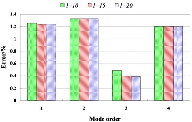
a) For lower bounds

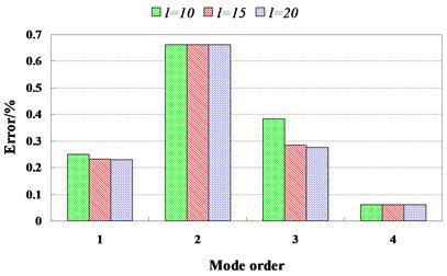
b) For upper bounds

6. Conclusions

1) An improved free interface CMS is proposed, which is easier to deal with the case with rigid body modes in component by constructing a set of weighted orthogonal modal vectors.

2) This paper provides a method for estimating the eigen solutions of the complicated system with uncertain properties at very little computational cost. In the first example, compared with the Monte Carlo method, the case study of a bridge structure proves that the component mode synthesis technique makes the process of non-deterministic analysis more efficiently without compromising the accuracy of the interval eigenvalue results. In the second example, the results obtained from the proposed method agree very well with the experimental results in natural frequencies. This shows the superior accuracy of the proposed method as well.