Abstract
This paper focuses on the fast highly approximate modal analysis and its applications in topology optimization design based on the triangle finite element. The proposed modal analysis methods are based on the initialized pseudo-random number vectors with the Rayleigh-Ritz analysis, which is very simple to implement and can easily be extended for structural dynamic topology optimization design. The numerical examples show that the proposed method is very effective with small computational cost and high efficiency which can effectively reduce huge computational cost without affecting the outcome of the optimization process. Meanwhile, the introduction of pseudo-random approximate modal analysis leads to the randomness and sub-optimal multiplicity of topology optimization results. Numerical examples show that the approximate pseudo-random modal analysis could also enlarge the search ability of the Optimality Criterion Method (OCM).
1. Introduction
In many large and complex structural systems, linear eigenvalue or modal analysis is important and appropriate for predicting modal response. However, in order to obtain the dynamic characteristic of huge structure, we usually directly calculate the Eigen-problem by QR algorithm or subspace iteration method [1]. Therefore, the computational cost may be too time consuming [2].
Since its introduction in the late 80 s, topology optimization has grown into a pervasive and versatile tool for designing structures for a wide variety of applications [3-8], which exhibits great advantages than the other material distribution design approach when a new design or material layout is sought for. Amir [9] pointed out, the solution is iterative and consists of repeated analyses followed by redesign steps in structural optimization. The high computational cost involved in repeated analyses of large-scale problems is one of the main obstacles in the solution process. The main drawback of topology optimization procedures is the added computational cost related to the multiple finite element analyses that should be performed within every design cycle. In fact, the modal or dynamic analysis is one of the main calculation work in structural topology optimization design especially for large-scale structure optimization design problem. Thus, how to greatly reduce the computational cost of modal analysis for structural topology optimization design becomes an interesting and important problem.
Presently, the modal or dynamic analysis for large-scale structure optimization design problem are rarely studied in the corresponding modal analysis or topology optimization design literature. The computational burden may be diminished by techniques that avoid the costly solution of multiple linear systems [9], which is just extended into robust topology optimization procedures for static analysis by Combined Approximations (CA) approach. So, the effective modal analysis techniques into topology optimization procedures is one of the main concern of this article, the other is the simplification and flexible multiplicity solutions of topology optimization. The aims are to approximate the eigensolution with a good level of precision and to reduce the global CPU time especially for dynamic analysis of large-scale structures and its applications in topology optimization design. Thus, the proposed analysis method could be a unified and efficient modal analysis method in huge structural analysis or topology optimization design.
As for the large structural modal analysis problem, the computational effort is significantly reduced by the proposed approximate modal analysis approach. The modal analysis procedure is easy to implement and could be integrated into an optimization process to improve its computational efficiency. Moreover, the introduction of pseudo-random number approximate dynamic analysis leads to the randomness and sub-optimal multiplicity of optimization results, which could provide several sub-optimal topology configurations for engineering applications. Section 2 briefly introduces the Eigen-equations for dynamic analysis problem. Section 3 describes the proposed modal analysis method with its steps, and simply test it by a modal analysis examples. Section 4 gives out the approximate formula to evaluate the possible saving of computational cost for the proposed modal analysis method. Section 5 introduces in detail the optimization modeling and optimization algorithm for structural topology optimization design based on the triangle finite element. Section 6 discusses the efficiency of the proposed method in terms of the precision and the CPU time by four numerical examples. Section 7 summarizes our conclusions.
2. Eigen-equation of analytical structure
2.1. Eigen-problem of structure
Firstly, the eigen-problem of linear analytical structure is given out in this section.
In finite element analysis (FEA), the natural vibration of undamped structure with DOF (degrees of freedom) leads to a general algebraic Eigen-problem:
where , , and are the stiffness matrix, the mass matrix, the th eigenvalue and th normalized eigenvector of the linear structure, respectively.
Here, we didn’t directly solve the Eq. (1), justly utilize the whole assembly stiffness and mass matrix and in modal analysis procedure.
3. The new structural modal analysis method based on pseudo random number vector for construction of initial basis vector
Usually, repeated analysis, or reanalysis, is needed in various problems of structural analysis, design and optimization. Reanalysis methods are intended to analyze efficiently structures that are modified due to various changes in their properties [10]. However, reanalysis methods are not easily extended into topology optimization design because the finite element mesh or DOF of the optimized structure is changed within every design cycle. Thus, we proposed a very simple modal analysis technique to calculate the approximate eigenvalues of the optimized structure. The technique consists of introducing the pseudo random number vectors to construct orthogonal basis vectors. Then the solution will converge to the highly approximate lower-order eigenvalues for the optimized structure by using Rayleigh-Ritz analysis. Jia [12] pointed out, there are always Ritz values that converges to the eigenvalues of the approximate problem. Obviously, the proposed modal analysis in topology optimization design become so easy to implement.
The proposed modal analysis method is divided into two simple steps as follow:
Step 1: pseudorandom number vector generation for initial orthogonal basis vector.
In first step, the proposed modal analysis method is to determine zero-order eigenvector by pseudorandom number vector generation, the equation is expressed as:
where is the element of the th initial eigenvector for analytical structure; is denoted as the number of initial basis vectors, is denoted as the number of FE (Finite Element) DOF for the structure; is the pseudorandom number generator, which means every component of the original eigenvector is a random number obey uniform distribution or normal distribution. By using this technique, we can easily construct the initial orthogonal basis vector for the following Rayleigh-Ritz analysis.
Step 2: Rayleigh-Ritz analysis.
In second step, we use Ritz procedure to evaluate the final and highly approximate eigen-matrixes (, ) for the computed structure.
(1) Execute the inverse iteration as follow:
(2) Calculate the projection based on the basis vectors from Eq. (3):
(3) Implement the Rayleigh-Ritz analysis:
(4) The final and highly approximate eigenvalues or eigenvectors are evaluated by:
and:
where, are only the several lower-order eigenvectors matrix for calculated structure. Usually, because we just need the several lower-order eigenvalues and eigenvectors by dynamic analysis for general engineering applications. As shown in the Section 3 by from Eq. (1) to Eq. (6), it is not an iteration process, and is finished by one computation for one optimization iteration step. Also, obviously, the proposed modal analysis procedure is very simple to implement and to be integrated into an optimization process to improve its computation efficiency.
In the following, by considering a transmission tower structure with 508 beam elements, shown in Fig. 1.
As assumed that the relative error of approximate eigenvalue calculated by the proposed modal analysis method (PMAM for short) compared to the exact eigenvalue by the OR algorithm is smaller than 0.1 or 10 percent, then the approximate eigenvalue is adequately approximate to the exact eigenvalue, the results for frequencies comparisons of the transmission tower structure by the two approaches are shown in Table 1.
As shown in Table 1, the average computational time of exact calculation by using the direct analysis method is 0.1429 seconds; and the average computational time by the proposed modal analysis method is 0.007512 seconds. Thus, the computational cost of modal analysis can be reduced by at least 94.74 % while maintaining sufficient accuracy.
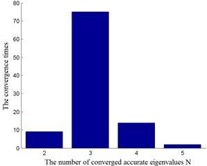
The approximate modal analysis was executed one hundred times calculations for the same structure (As similar to the Subspace iteration method [1], we choose several original vectors, and then we will obtain the several lower-order eigenvalues by the proposed modal analysis method. Here, the number of the original basis vector is usually equal to six or eight). Although the approximate solution is pseudorandom, we found the lower-order approximate eigenvalues converged to the accurate eigenvalues in this numerical experiment with great probability (nearly 90 percentage), which is shown in Fig. 2.
Table 1The comparisons between the approximate frequencies and the exact frequencies
Frequency (Hz) | Exact (calculated by QR) | Approximate (calculated by PMAM) | Relative error |
1 | 0.8197 | 0.8514 | 0.0387 |
2 | 0.9080 | 0.9212 | 0.0145 |
3 | 0.9739 | 1.0223 | 0.0497 |
4 | 1.3038 | 1.3593 | 0.0426 |
5 | 1.3560 | 1.4379 | 0.0604 |
6 | 2.4722 | 4.6935 | 0.8985 |
The actual computational cost | 0.1429 s | 0.007512 s |
Fig. 1The transmission tower structure
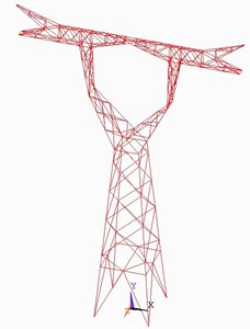
Fig. 2The convergence times for different number of accurate eigenvalues
4. Discussions about the general saving of computational cost for the proposed approximate modal analysis method
Executing by Fortran or Matlab code, the whole running time of the approximate modal analysis was measured relatively to the whole running time of standard FE direct solve in modal analysis or topology optimization design with various FE mesh sizes. In the approximate analysis schemes, the major calculation cost is due to the computation of inverse iteration in Eq. (3). Denoting as the number of degrees of freedom for the analyzed structure, is the number of the needed approximate eigenvalues (Assuming that the value of b is usually less than four); for the general real case, the overall cost is roughly operations if only the eigenvalues are needed by the direct dynamic analysis method for every design cycle, and the computational cost of approximate modal analysis is proportional to operations [13-16]. Thus, the approximate saving of computational cost for the proposed modal analysis method is generally expressed as:
Fairly rough outcome by approximate dynamic analysis will be achieved for the computational cost of around 10 % compared to a direct solve, which is based on the simple calculation of Eq. (7). The accurate saving of the approximate modal analysis method will be examined in several topology optimization design experiments.
5. The modeling and optimization algorithm for structural topology optimization design based on the optimality criterion method
5.1. The mathematical model for structural topology optimization design
By considering the displacement constraint and frequency constraint, the mathematical model of topology optimization design problem can be formulated as:
where is the objective function (to minimize the structure mass), and are the element density and volume, respectively; , are the actual displacement and the upper bound of the constrained displacement for the appointed DOF, respectively; and are the actual th frequency and the lower bound of the th constrained frequency for the optimized structure; is the topology design variable, and are the lower bound and upper bound of the topology design variable , respectively.
5.2. The iteration formula for topology design variable based on the displacement sensitivity analysis
By using Eq. (8), we could construct the approximate Lagrange function:
where is the Lagrange multiplier.
By derivation of both sides of Eq. (9) with respect to the design variable , and making the derivatives is equal to zero, we can obtain:
Assuming:
We can obtain the iteration formula as follow:
where is the relaxation factor, and is denoted as iteration step. Usually, can be calculated by virtual load displacement sensitivity analysis method.
By considering the single displacement constraint condition, and we take the derivatives of the both sides of the FE equilibrium equation with respect to the design variable . And assuming that the right-hand side is independent to the design variable , we can obtain:
By multiplying for both sides of Eq. (13), and summing all the equations, we can obtain:
In general case for 2D, the element stiffness matrix could be expressed as the following form:
where is only related to the element shape and material. Thus, we can obtain the following equations:
By substituting the Eq. (16) into Eq. (14), and we take the displacement component corresponding to the constrained displacement for the appointed DOF, we can obtain:
By multiplying for both sides of Eq. (9) and considering the Eq. (17), and summing the equations; meanwhile, when it is the optimal solution, we have , Thus, as for plane elastic plate problem, the Lagrange multiplier can be obtained by the following equation:
Similarly, for the bending thin plate problem, the Lagrange multiplier can be obtained by the following equation:
5.3. The iteration formula for the topology design variable based on the frequency sensitivity analysis
Assuming that the arbitrary order eigenvector is corresponded to the eigenvalue , then the structural eigen-problem corresponding to the free vibration can be expressed as:
where and are the structural stiffness matrix and mass matrix, respectively. They are assembled by element stiffness and element mass matrix as follow:
where and are denoted as the element stiffness matrix and mass matrix, respectively.
By calculating the differential of the both sides for Eq. (20) with respect to the design variable , we can have:
where subscript is denoted as the partial differential with respect to the design variable .
By multiplying for both sides of Eq. (22), and making the left side is equal to zero, we can obtain:
By considering the single frequency constraint problem, the frequency constraint is usually described as:
where is the lower bound of the constrained frequency.
Here, the Lagrange function can be approximately expressed as:
By utilizing the Kuhn-Tucker condition with some approximation and simplifications, the iteration formula based on frequency sensitivity analysis can also expressed as [10]:
where is denoted as element mass parameter, and is the Lagrange multiplier, (0.001, 0.4), (0.6, 1.6). Generally, we set the parameter and to be the maximal value in the numerical examples.
5.4. The continuum topology optimization design algorithm based on ICM (Independent, Continuous and Mapping) or SIMP method [17, 18 and 19]
Now, we utilize the hybrid ICM and SIMP method to solve the problem in Eq. (8). There exist three filter function in ICM method, which are expressed as:
where , and are the element weight, element stiffness matrix and element mass matrix filter functions, respectively. We can find the detailed ICM algorithm flowchart in literature [17, 18], which is omitted here.
5.4.1. Independent sensitivity filter [19]
Firstly, in order to avoid the general numerical unstable phenomenon in topology optimization such as checkerboard and mesh dependence, we use the independent sensitivity filter method to obtain clear and smooth topology configuration.
Assuming the displacement sensitivity variable and frequency sensitivity variable are denoted as and , respectively, we compute the element weight factor ( 1, 2,…, ) as follow:
where is denoted as the filter characteristic radius, is described as the center distance between the element and element. Then the displacement sensitivity variable for element after filter is computed as follow:
Similarly, the frequency sensitivity variable for element after filter is expressed as:
By substituting and into the Eq. (12) and Eq. (26), respectively, we could obtain the renew topology design variable .
In order to ensure the convergence of topology optimization design, we utilize the regulation strategy. Assuming the renew topology design variable after filter are expressed as and , then the regulated topology design variable is calculated as follow:
where is used for calculating the median value of topology optimization design variable vector.
5.4.2. Filter treatment based on sensitivity redistribution [11]
Secondly, for further eliminating the checkerboard in topology optimization design, we utilize the sensitivity redistribution to filter the design variable .
(1) Firstly, the nodal design variable is calculated as follow:
where is denoted as nodal design variable, which is used as transition variable; is expressed as the element number that is connected to the node.
(2) Secondly, the new topology design variable is expressed as:
where is the number of nodes for per element.
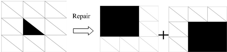
5.4.3. Repair strategy for eliminating the checkerboard phenomenon
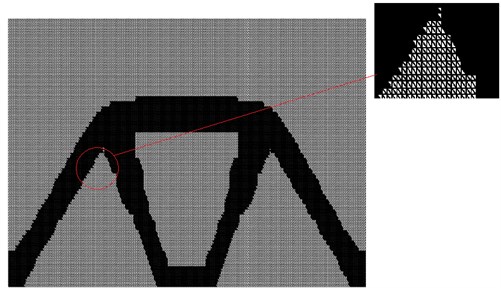
Usually, the resultant topology formed is inconsistent or not desirable [20]. Finally, we utilize repair strategy to eliminate the checkerboard phenomenon. The repair strategy is shown in Fig. 3.
Obviously, this simple repair strategy could effectively be eliminating the checkerboard phenomenon or inconsistent section in topologies.
Fig. 3The repair strategy for eliminating the checkerboard
5.4.4. Strategy of two-terminal division based on average value
Finally, in order to speed up the convergence process of topology optimization design, we utilize the strategy of two-terminal division based on average value as follow:
where (0.1, 0.3) is denoted as moving step, here we set the value of this parameter to be 0.1 in examples; is the renew topology design variable, is the Signum function, is expressed as the mean function.
5.4.5. Convergence criterion for topology optimization design
The convergence criterion of topology optimization design is defined as:
where and are the values of objective function for the step iteration and step iteration, respectively.
Now, the whole modeling and optimization algorithm for structural topology optimization design is given out in Section 5. Although the presented optimization algorithm above is slightly hybrid and coarse, but its validity and efficiency are certified in Section 6. In essence, the algorithm basis of the proposed optimization method is Optimality Criterion Method (OC method), thus the it always converges to the approximate optimal solution after several iterations [21].
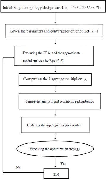
5.4.6. The implementation details or procedure of the optimization algorithm
The procedure of the optimization algorithm is concluding as follow:
(a) Initializing the topology design variable, 0.1, ( 1, 2,…, );
(b) Given , , and other parameters, let , , (1, 2,…, );
(c) Executing the FEA, and the approximate modal analysis by Eqs. (2-6);
(d) Computing the Lagrange multiplier ;
(e) Executing the displacement sensitivity analysis and sensitivity redistribution, frequency sensitivity analysis and sensitivity redistribution;
(f) Updating the topology design variable and filter treatment by Eqs. (32-34);
(g) If the convergence criterion is met, stopping the optimization iteration or optimization is ended; else let , , (1, 2,…, ) return to step (c);
The whole procedure of the optimization algorithm is also shown in Fig. 4.
Fig. 4The flowchart of the optimization algorithm
6. Numerical examples
To test the proposed approximate modal analysis method, we use four topology optimization numerical examples. The optimization algorithm is used by hybrid ICM and SIMP method from literature [11, 18, 19], and executed by MATLAB procedure based on literature [19]. The main concern of this article is to deal with the low efficiency problem of direct modal analysis in topology optimization. For comparisons, the exact modal analysis is used by QR algorithm in commercial software for topology optimization design; the approximate modal analysis is used by the proposed method in Section 2.
Example 1: Considering the base structure as a rectangle bending plate structure, shown in Fig. 5, with its material and structural parameters given by: elasticity modulus is 2.1×10¹¹Pa, the thickness of plate is 0.1 m, mass density is 7.80×10³ kg/m3, the Poisson’s ratio is equal to 0.3, the length and width of plate are 6 m and 6 m, respectively.
Fig. 5The base structure of the around clamped boundary bending plate structure
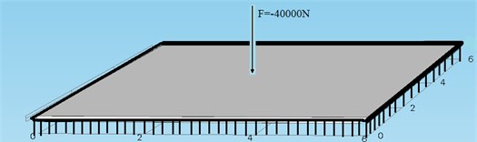
The clamped boundary base structure is discretized into 120×240 triangle plate elements. The down-ward external force with 40000 N is applied on the middle point of the structure. The termination criteria tolerance of topology optimization design is 0.0001. The maximum allowable midpoint deflection was constrained to 0.001 m. The frequency constraint is that the first natural frequency of the optimal structure is not less than 18 Hz.
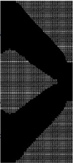
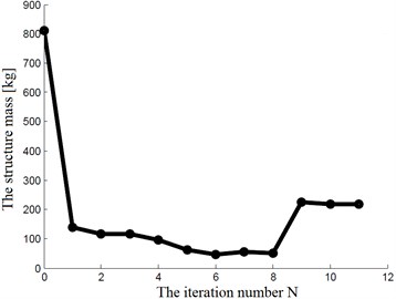
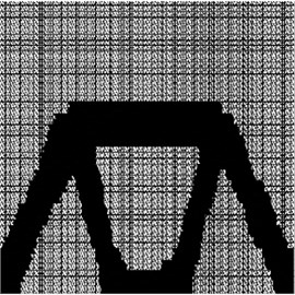
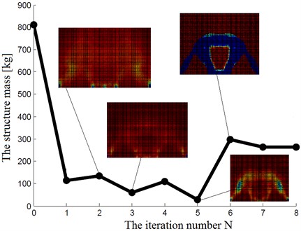
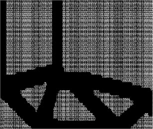
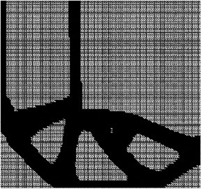
Fig. 6. shows the optimal topology structure, and the iteration history of the objective function mass is shown as Fig. 7.
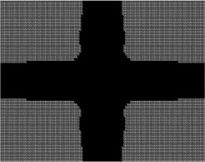
Fig. 6The optimal structure topology
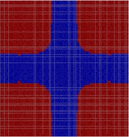
Fig. 7The iteration history of structure mass
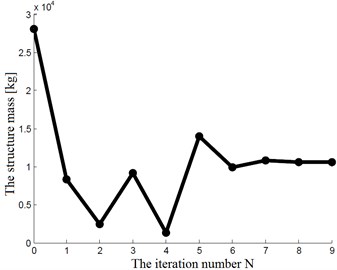
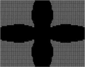
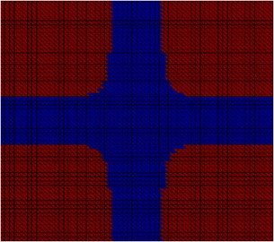
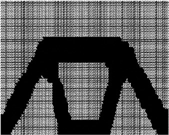
Fig. 8The sub-optimal topology structures by the proposed dynamic analysis method
a)
b)
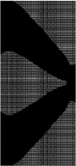
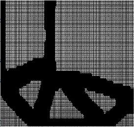
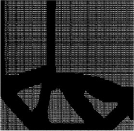
The deflection of middle point for the optimal structure is 0.000986 m, the first natural frequency of the optimal structure is 18.1026 Hz. Thus, the optimal results satisfy all the constraints. For comparison, we have also included plots of the several sub-optimal topology structures with the optimal structure based on the direct dynamic analysis method (DAM), as shown in Fig. 8 and Fig. 9. The iteration history of structure mass by the proposed optimization method based on the direct modal analysis method is also shown in Fig. 10.
Fig. 9The optimal topology structure by the direct dynamic analysis method
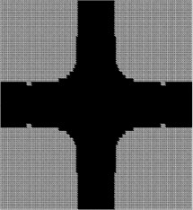
Fig. 10The iteration history of structure mass by the proposed optimization method based on the direct modal analysis method
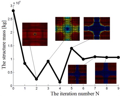
As shown in Fig. 10, there exactly exist the grey zones at the beginning of the optimization process, but the grey zones quickly disappear at the subsequent optimization iteration steps.
In order to verify the mesh-independency of the proposed method, we show some other optimization result under different mesh for example 1 in Fig. 11.
Fig. 11The optimal structure topology under different mesh (mesh 60×120)
As shown in Fig. 11, the optimal structure topology is similar under different mesh.
The comparisons between the approximate eigenvalues and the exact eigenvalues are shown in Table 2.
Obviously, the eigenvalues calculated by the approximate modal analysis are much approximate to the eigenvalues calculated by the exact analysis.
The optimization results comparison by the optimization method based on the approximate modal analysis and the optimization method based on the exact analysis are shown in Table 3.
Table 2The comparisons between the approximate eigenvalues and the exact eigenvalues
Eigenvalue | Exact (calculated by QR) | Approximate (calculated by PMAM) | Relative error |
1 | 1.596E+4 | 1.555E+4 | 0.0257 |
2 | 8.41E+4 | 8.32E+4 | 0.0107 |
3 | 8.41E+4 | 8.66E+4 | 0.0297 |
4 | 2.23E+5 | 2.22E+5 | 0.00448 |
5 | 4.11E+5 | 4.34E+5 | 0.0560 |
6 | 4.64E+5 | 5.18E+5 | 0.116 |
Table 3The optimization results comparison by the two method
Frequency / Hz | Displacement / m | Mass / Kg | Iterations / number | |
Exact analysis optimization method | 18.24 | 9.86×10⁻⁴ | 11128 | 9 |
Approximate analysis optimization method | 18.26 | 9.86×10⁻⁴ | 11150 | 0 |
As shown in the Table 3, the optimization results are approximate for the two optimization method.
Here, with the same computational platform and computational environment, the comparisons of the computational cost for the standard direct dynamic analysis and the approximate dynamic analysis in topology optimization design are as follow: the average time of exact calculation by using the direct method is 79.6574 seconds; and the average computational time by the proposed dynamic analysis method is 8.0320 seconds. Thus, the computational cost of modal analysis can be reduced by at least 89.92 % while maintaining sufficient accuracy.
Example 2: Considering the base structure as a plane stress structure, shown in Fig. 12, with its material and structural parameters given by: elasticity modulus is 6.889×10¹⁰Pa, the thickness of plate structure is 0.009 m, mass density is 1.0×10⁴ kg/m3, the Poisson’s ratio is equal to 0.3, the length and width of plate are 0.1 m and 0.24 m, respectively.
Fig. 12The base structure of the left boundary clamped plane stress plate
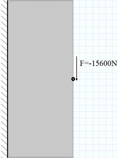
The left boundary clamped base structure is discretized into 160×192 triangle plane stress elements. The down-ward external force with 15600 N is applied on the middle point of the right-hand. The termination criteria tolerance of topology optimization design is 0.0001. The maximum allowable midpoint displacement was constrained to be 0.00015 m. The frequency constraint is that the first natural frequency of the optimal structure is not less than 3000 Hz.
Fig. 13 shows the optimal topology structure, and the iteration history of the objective function mass is shown as Fig. 14.
Fig. 13The optimal structure topology
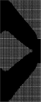
Fig. 14The iteration history of structure mass
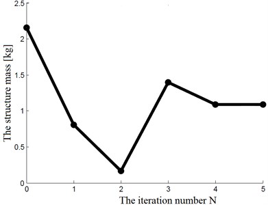
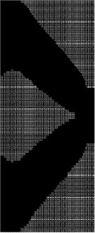
The displacement of the middle point for the optimal structure is 0.0001486 m, the first natural frequency of the optimal structure is 3185.381 Hz. Thus, the optimal results satisfy all the constraints. For comparison, we have also included plots of the several sub-optimal topology structures with the optimal structure by the direct dynamic analysis method, as shown in Fig. 15 and Fig. 16. The iteration history of structure mass by the proposed optimization method based on the direct modal analysis method is also shown in Fig. 17.
Fig. 15The sub-optimal topology structures by the proposed dynamic analysis method
a)
b)
Fig. 16The optimal topology structure by the direct dynamic analysis method
In order to verify the mesh-independency of the proposed method, we show some other optimization results under different mesh for example 2 in Fig. 18.
As shown in Fig. 18, the optimal structure topology is similar under different mesh.
The comparisons between the approximate eigenvalues and the exact eigenvalues are shown in Table 4.
Here, with the same computational platform and computational environment, the comparisons of the computational cost for the standard direct dynamic analysis and the approximate dynamic analysis in topology optimization design are as follow: the average time of exact calculation by using the direct dynamic analysis method is 5.6691 seconds; and the average computational time by the proposed dynamic analysis method is 1.0356 seconds. Thus, the computational cost of modal analysis can be reduced by at least 81.83 % while maintaining sufficient accuracy.
Fig. 17The iteration history of structure mass by the proposed optimization method based on the direct modal analysis method
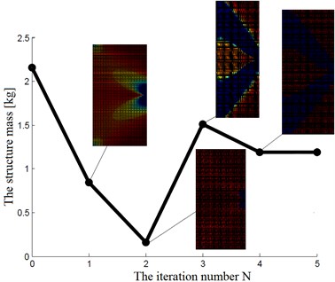
Fig. 18The optimal structure topology under different mesh (mesh 96×80)
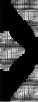
Table 4The comparisons between the approximate eigenvalues and the exact eigenvalues
Eigenvalue | Exact (calculated by QR) | Approximate (calculated by PMAM) | Relative error |
1 | 3.59E+8 | 3.54E+8 | 0.014 |
2 | 7.93E+8 | 7.77E+8 | 0.0202 |
3 | 1.30E+9 | 1.33E+9 | 0.0230 |
4 | 1.72E+9 | 1.79E+9 | 0.0407 |
5 | 2.46E+9 | 2.58E+9 | 0.0487 |
6 | 2.81E+9 | 3.00E+9 | 0.0676 |
Example 3: Considering the base structure as a plane stress structure, shown in Fig. 19, with its material and structural parameters given by: elasticity modulus is 6.889×10¹⁰Pa, the thickness of plate structure is 0.006 m, mass density is 1.0×10⁶ kg/m3, the Poisson’s ratio is equal to 0.3, the length and width of plate are 0.52 m and 0.26 m, respectively. The left and right corner points at the bottom end are fixed. The boundary and load condition are as shown in Fig. 19. The base structure is discretized into 208×52 triangle elements. The termination criteria tolerance of topology optimization design is 0.0001. The maximum allowable displacements in point 1, 2, and 3 were constrained to be 0.0009 m, 0.001 m and 0.0009 m, respectively. The frequency constraint is that the first natural frequency of the optimal structure is not less than 19 Hz.
Fig. 20. shows the optimal topology structure, and the iteration history of the objective function mass is shown as Fig. 21.
Fig. 19The base structure of the plane stress plate
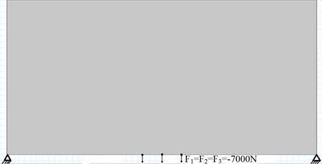
Fig. 20The optimal structure topology
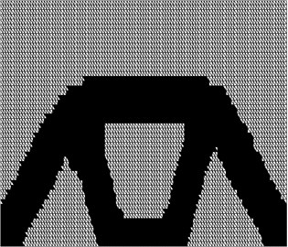
Fig. 21The iteration history of structure mass
The displacements of the three points for the optimal structure are 0.000889 m, 0.001 m and 0.000889 m, respectively. The first natural frequency of the optimal structure is 20.618 Hz. Thus, the optimal results satisfy all the constraints. For comparison, we have also included plots of the several sub-optimal topology structures with the optimal structure by the direct dynamic analysis method, as shown in Fig. 22 and Fig. 23. The iteration history of structure mass by the proposed optimization method based on the direct modal analysis method is also shown in Fig. 24.
Fig. 22The sub-optimal topology structures by the proposed dynamic analysis method
a)
b)
Fig. 23The optimal topology structure by the direct dynamic analysis method
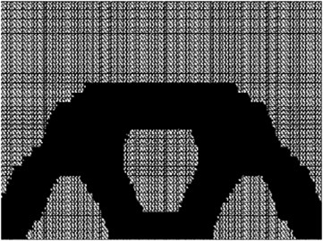
Fig. 24The iteration history of structure mass by the proposed optimization method based on the direct modal analysis method
In order to verify the mesh-independency of the proposed method, we show some other optimization result under different mesh for example 3 in Fig. 25.
The comparisons between the approximate eigenvalues and the exact eigenvalues are shown in Table 5.
Fig. 25The optimal structure topology under different mesh (mesh 104×416)
Here, with the same computational platform and computational environment, the comparisons of the computational cost for the standard direct dynamic analysis and the approximate dynamic analysis in topology optimization design are as follow: the average time of exact computation by using the direct method is 2.8534 seconds; and the average computational time by the proposed modal analysis method is 0.5633 seconds. Thus, the computational cost of dynamic analysis can be reduced by at least 80.26 % while maintaining sufficient accuracy.
Table 5The comparisons between the approximate eigenvalues and the exact eigenvalues
Eigenvalue | Exact (calculated by QR) | Approximate (calculated by PMAM) | Relative error |
1 | 1.71E+4 | 1.68E+4 | 0.0175 |
2 | 1.82E+5 | 1.82E+5 | 0.0022 |
3 | 6.97E+5 | 6.97E+5 | 0.00086 |
4 | 9.15E+5 | 8.94E+5 | 0.0230 |
5 | 1.22E+6 | 1.20E+6 | 0.0201 |
6 | 1.62E+6 | 1.60E+6 | 0.0143 |
Example 4: Considering the base structure as a L-shape plane stress structure, shown in Fig. 26, with its material and structural parameters given by: elasticity modulus is 6.889×10¹⁰Pa, the thickness of plate structure is 0.009 m, mass density is 1.0×04 kg/m3, the Poisson’s ratio is equal to 0.3, the length and width of plate are shown in Fig. 26.
Fig. 26The base structure of the plane stress plate
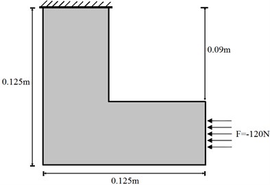
The upper boundary clamped base structure is discretized into 12800 triangle elements. The distribution external force with –120 N is applied on the right-hand, as shown in Fig. 26. The termination criteria tolerance of topology optimization design is 0.0001. The maximum allowable midpoint displacement was constrained to be 0.0002 m. The frequency constraint is that the first natural frequency of the optimal structure is not less than 450 Hz.
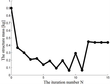
Fig. 27. shows the optimal topology structure, and the iteration history of the objective function mass is shown as Fig. 28.
Fig. 27The optimal structure topology
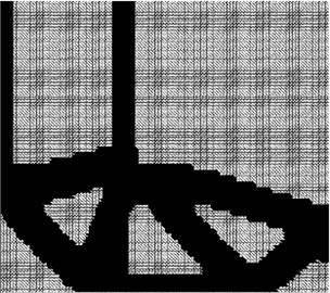
Fig. 28The iteration history of structure mass
The displacements of the midpoint for the optimal structure are 0.0001998 m. The first natural frequency of the optimal structure is 468.48 Hz. Thus, the optimal results satisfy all the constraints. For comparison, we have also included plots of the several sub-optimal topology structures with the optimal structure by the direct dynamic analysis method, as shown in Fig. 29 and Fig. 30.
Fig. 29The sub-optimal topology structure by the proposed dynamic analysis method
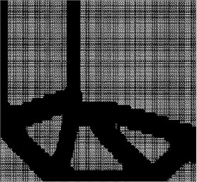
a)
b)
Fig. 30The optimal topology structures by the direct dynamic analysis method
The iteration history of structure mass by the proposed optimization method based on the direct modal analysis method is also shown in Fig. 31.
We also compared the optimization results based on the triangle elements with the optimization results based on the rectangular elements, which is shown in Fig. 32.
Fig. 31The iteration history of structure mass by the proposed optimization method based on the direct modal analysis method
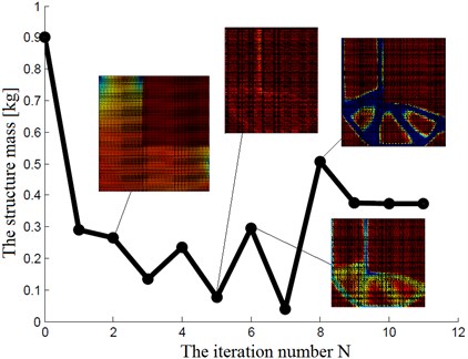
Fig. 32The optimal structure topology based on the rectangular finite elements
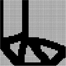
Fig. 33The optimal structure topology based on the sparse pseudorandom initialization
Obviously, the optimal structure topology is similar to each other for the rectangular elements and the triangle elements.
In order to verify the mesh-independency of the proposed method, we show some other optimization result under different mesh for example 4 in Fig. 34.
Fig. 34The optimal structure topology under different mesh (mesh 150×300)
Here, with the same computational platform and computational environment, the comparisons of the computational cost for the standard direct dynamic analysis and the approximate dynamic analysis in topology optimization design are as follow: the average time of exact computation by using the direct method is 9.0649 seconds; and the average computational time by the proposed modal analysis method is 2.6202 seconds. Thus, the computational cost of dynamic analysis can be reduced by at least 71.09 % while maintaining sufficient accuracy.
The Table 6, shows the actual savings of computational cost for the four numerical examples by the proposed dynamic analysis (DA) method.
Table 6The actual savings of computational cost for the four numerical examples by the proposed dynamic analysis method
The computational cost by standard DA (s) | The computational cost by approximate DA (s) | The saving of computational cost (percentages) | |
Example 1 | 79.6574 | 8.0320 | 89.92 % |
Example 2 | 5.6691 | 1.0356 | 81.83 % |
Example 3 | 2.8534 | 0.5633 | 80.26 % |
Example 4 | 9.0649 | 2.6202 | 71.09 % |
Clearly, the benefit of applying approximate modal analysis techniques increases with the increase of FE mesh sizes within a single optimization cycle. Examining the optimized layouts, the goals of topology optimization design are satisfied despite the minor difference in performance between the optimal design by the proposed dynamic analysis procedure and the optimal structure by the standard dynamic analysis procedure. A thorough examination of the prospects of such an approximate dynamic analysis approach is left for future work, but some promising results are given in the above.
7. Conclusions
The paper focuses on the structural modal analysis for topology optimization design based on the triangle finite element. An efficient modal analysis approach to topology optimization design was presented. The high computational effort of solving dynamic equation is decreased by utilizing approximate modal analysis procedures. According to numerical experiments, the computational cost of dynamic analysis can be reduced by at least 70 % while maintaining sufficient accuracy. The extent of the actual savings depends on the properties of the problem in hand as well as on the efficiency of the computer code. Based on the results of the current study as well as on the conclusions of previous investigations, we believe that the key for deriving dynamic analysis procedures that yield sufficient accuracy for minimal computational cost lies in linking dynamic analysis and optimization. This means that ultimately, the required accuracy of dynamic analysis will be defined rigorously within the optimization routine according to the progress of optimization [8].
References
-
Bathe K. J. The subspace iteration method – revisited. Computers and Structures, Vol. 126, 2013, p. 177-183.
-
Massa F., Lallemand B., Tison T. Multi-level homotopy perturbation and projection techniques for the reanalysis of quadratic eigenvalue problems: the application of stability analysis. Mechanical Systems and Signal Processing, Vol. 52, Issue 53, 2015, p. 88-104.
-
Xu B., Ou J. P., Jiang J. S. Integrated optimization of structural topology and control for piezoelectric smart plate based on genetic algorithm. Finite Elements in Analysis and Design, Vol. 64, 2013, p. 1-12.
-
Xiaopeng Zhang, Zhan Kang Dynamic topology optimization of piezoelectric structures with active control for reducing transient response. Computer Methods in Applied Mechanics and Engineering, Vol. 281, 2014, p. 200-219.
-
Kai James A., Haim Waisman Topology optimization of viscoelastic structures using a time-dependent adjoint method. Computer Methods in Applied Mechanics and Engineering, Vol. 285, 2015, p. 166-187.
-
Lei Li, Kapil Khandelwal Volume preserving projection filters and continuation methods in topology optimization. Engineering Structures, Vol. 85, 2015, p. 144-161.
-
Jaejong Parka, Alok Sutradhar A multi-resolution method for 3D multi-material topology optimization. Computer Methods in Applied Mechanics and Engineering, Vol. 285, 2015, p. 571-586.
-
Asger Nyman Christiansenn, Andreas Bærentzen J., Morten Nobel-Jørgensen, et al. Combined shape and topology optimization of 3D structures. Computers and Graphics, Vol. 46, 2015, p. 25-35.
-
Oded Amir, Ole Sigmund, Boyan Lazarov S., et al. Efficient reanalysis techniques for robust topology optimization. Computer Methods in Applied Mechanics and Engineering, Vols. 245-246, 2012, p. 217-231.
-
Kirsch U. Reanalysis of Structures – A Unified Approach for Linear, Nonlinear, Static and Dynamic Systems. Springer, Dordrecht, 2008.
-
He Jianjun, Jiang Jiesheng Hybrid method of topology optimization for continuum structures based on displacement and frequency constraints. Chinese Journal of Mechanical Strength, Vol. 30, Issue 6, 2008, p. 941-946.
-
Zhongxiao Jia, Stewart G. W. An analysis of the Rayleigh-Ritz method for approximating eigenspaces. Mathematics of Computation, Vol. 70, Issue 234, 1999, p. 637-647.
-
Parlett B. N. The QR algorithm. Computing in Science and Engineering, Vol. 2, Issue 1, 2000, p. 38-42.
-
Wilkinson J. H. The Algebraic Eigenvalue Problem. Oxford University Press, New York, 1965.
-
Stewart G. W. The decompositional approach to matrix computation. Computing in Science and Engineering, Vol. 2, Issue 1, 2000, p. 50-59.
-
Mathews J. H., Fink K. D. Numerical Methods Using Matlab. 3d Edition, Prentice Hall, Upper Saddle River, NJ, 1999.
-
Sui Yunkang, Yang Deqing A new method for structural topological optimization based on the concept of independent continuous variables and smooth model. Acta Mechanica Sinica, Vol. 14, Issue 2, 1998, p. 179-185.
-
Sui Y. K., Ye H. L., Peng X. R. Topological optimization of continuum structure with global stress constraints based on ICM method. Computational Methods, 2006, p. 1003-1014.
-
Sigmund O. A 99 line topology optimization code written in Matlab. Structural and Multidisciplinary Optimization, Vol. 21, 2001, p. 120-127.
-
Faez Ahmed, Kalyanmoy Deb, Bishakh Bhattacharya Structural topology optimization using multi-objective genetic algorithm with constructive solid geometry representation. Applied Soft Computing, Vol. 39, 2016, p. 240-250.
-
Dheeraj Gunwant, Anadi Misra Topology optimization of continuum structures using Optimality criterion approach in ANSYS. International Journal of Advances in Engineering and Technology, Vol. 5, Issue 1, 2012, p. 470-485.
About this article

The authors would like to thank for the supports by Natural Science Foundation of China under grant 51305048, 11372249, 51408069, and Scientific Research Fund of Hunan Provincial Education Department under Grant 11C0045.
