Study of double-potential-well leaf spring system’s chaotic vibration

1. Introduction

Chaos has become increasingly popular in resolving complicated problems in engineering fields [1]. On one hand, a lot of projects have been conducted to identify and understand chaotic behaviors in a system and try to reduce the influence from chaos. Gao et al. developed a self-adaptive tracking control system to constrain large amplitude chaotic motion occurred in a motor suspension system [2] and Han et al developed a sliding mode controlling method to reduce Lorenz chaotic vibration [3]. On the other hand, some engineering solutions/designs were trying to take advantage of a system’s chaotic behavior and deliberately introduce chaos to improve the system’s efficiency. For example, Long et al. invented a chaotic vibration roller which significantly increased the device’s working efficiency [4]. DMITRIEV et al study the speech and music signal transmission by chaos [5]. Govindan R. B. et al. applied chaos theory to diagnose the patient ECG [6].

As an important component, leaf springs have long been used in the suspension system of wheeled vehicles. Recent development is considering nonlinear vibration in the design of leaf springs to improve the system’s reliability. The nonlinear large deformation, contact and friction are usually applied to characterize the nonlinear behavior of leaf springs. OMAR et al. [7] researched a nonlinear finite-element procedure to accurately model the deformations and vibrations of the leaf springs, in which the effect of the distributed inertia and elasticity are considered. Qing Li et al studied the multileaf spring in vehicles and develop a contact finite element algorithm. Then, a piecewise contact stress pattern is approximated to the original contact state between two layered beams [8]. Yong-Jin Yum researched the frictional characteristics of automotive leaf spring. The load-strain results of the compression test are obtained, and the finite element analysis was used to calculate the friction force [9]. Hiroyuki Sugiyama et al present a nonlinear elastic model of leaf springs to simulate the multibody vehicle systems. The nonlinear dynamic coupling between the finite rotations and the leaf deformation are analyzed, and the leaf spring geometry and deformations are modelled with the distributed inertia and stiffness [10].

Because the leaf spring has the same structure dynamics as the beam, it is beneficial to design and analyze spring base on the beam theory, and the analogous complex behavior of beam will occur in the leaf spring. Rahman et al designed a parabolic leaf spring, and used both the small and large deflection theories to calculate the stress and the deflection of the beam, in which the geometric nonlinearity is analyzed [11]. Dwivedy et al. investigate the nonlinear response of a base-excited slender beam carrying an attached mass, and the fixed-point, periodic, quasiperiodic and chaotic vibration are observed [12]. Nayfeh et al. studied the nonlinear dynamics of the fixed-free in extensional beam under the principal parametric excitation. The cubic nonlinearities due to the curvature and inertial are contained in the equations of motion. For some range of parameters, Hopf bifurcation exist, and response consists of amplitude and phase modulated or chaotic motions [13]. Li Chen proposed a moment integral treatment approach and applied it to the problems of complex and varying beam properties [14]. Nallathambi et al. developed an algorithm to analyze the large deflection of curved prismatic cantilever beams with uniform curvature subjected to a follower load at tip. The novel method reducing two-point boundary value problem to an initial value problem, and a single parameter shooting integrating strategy of the cantilever beam is develop [15].

Since the leaf spring undergoes large deflections when it is subjected to external excitation, the solutions of those highly nonlinear problems become very complex. Elliptic integral formulation [16], Galerkin procedure, R-K method with shooting technique [17, 18], finite difference method [19] and finite element method(FEM) [20] are the frequently used. Nayfeh et al. [21] applied the combination of Galerkin procedure and the method of multiple scales to construct a first-order uniform expansion for the inextensional beam. The results show that the nonlinear inertial terms produce a softening effect and play a significant role in the planar response of high frequency modes. Besides, the double potential well Duffing theory is used to research the nonlinear dynamics analytically. S. Li et al. used a self-excited term of Rayleigh type and Duffing double well potential to model vehicle suspension system due to electro- or magneto-rheological fluid damping where it is causing a hysteretic effect [22]. Thompson studied the manner of metastable mechanical oscillator escaping from cubic potential well. The basin of attraction is obtained, and he Melnikov method is applied to predict the homoclinic tangle [23]. Teueba et al. studied the nonlinearly damped double-well Duffing oscillator and analytically estimates how certain nonlinear damping terms affects the dynamics of the nonlinear oscillator. The condition of Melnikov-equivalence between the nonlinear damping system and the linear damping one is obtained [24]. Grzegorz Litak et al. introduced a harmonic excitation term and damping as perturbations, the critical Melnikov amplitude of the road surface profile is found, above which the system can vibrate chaotically [25].

Experimental studies for these systems are particularly important. However, few experimental studies have been carried out to investigate the chaos characteristics of leaf springs carefully. Liang Shan et al investigate the chaotic vibration of a vehicle model over road excitation [26]. Moon and Holmes investigated chaotic vibration of the beam in the magnetic field [27]. Fossas et al. studied the chaos in buck converter [28]. One common problem challenging all of these experimental studies is how to keep the system under a certain chaotic regime and produce stable and repeatable chaotic vibration. Besides, the signal processing methods are required to extract the chaotic characteristic effectively.

Therefore, in this paper, an experimental study was carried out to investigate the chaotic vibration of leaf springs. The natural frequencies where the chaotic vibration can be potentially excited were obtained from static analysis using a finite element based numerical model. The dynamic characteristics of the leaf spring were investigated experimentally on a test rig which was designed based on the double potential well theory [27]. A newly developed signal processing method, Wavelet-SG-EEMD )Wavelet, Savitzky-Golay (SG) and Ensemble Empirical Mode Decomposition(EEMD)) [29-32], were used to reduce noise and help to identify chaos features of the vibration signal generated by the system. A phase space reconstruction method, based on the first minimum mutual information (FMMI) theory, was used to obtain the chaotic attractors. An improved fast space grid algorithm [33] was used to obtain the maximum Lyapunov Exponent (LE) of the signal. A modified Poincaré method [34] was used to obtain the experimental Poincaré section.

In Section 2, the nonlinear amplitude and frequency characteristic curve of the double potential well system is analyzed, and the bifurcation is researched numerically. In Section 3, natural frequencies and relevant modes of the leaf spring used in the experiment are obtained by FE methods. In Section 4 the design of the leaf spring test rig is introduced. Details of Wavelet-SG-EEMD denoising method are presented in Section 5. Results from the experimental signals are analyzed and discussed in Section 6. Conclusions are given in Section 7.

2. Mechanism of the double-potential-well

2.1. Mathematic model

The differential equation of motion for the leaf spring system with magnets is simplified to double potential well system and it is modeled as the Duffing equation [27]:

1

$\ddot{z}+\xi \dot{z}+\gamma z+\beta z^3=f\mathrm{c}\mathrm{o}\mathrm{s}\left(\tilde{\omega }\tau \right),$

where $\xi$ is the dimensionless damping factor, $\gamma$ is dimensionless linear stiffness, $\beta$ is dimensionless nonlinear stiffness, $f$ is the dimensionless force amplitude, $\tilde{\omega }$ is dimensionless excitation frequency, $\ddot{z}=d^{2}z/d{\tau }^2$, $\dot{z}=dz/d\tau$. For the Eq. (1), the nonlinear restoring force of the spring is:

2

$F\left(z\right)=-\gamma z-\beta z^3.$

The potential function $V\left(z\right)$ is defined as:

3

$V\left(z\right)=\gamma z^2/2+\beta z^4/4.$

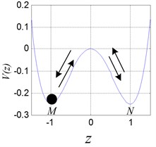
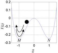
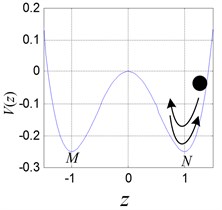
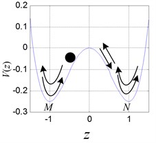
In Eq. (3), when the parameter $\gamma$ is –1, and $\beta$ is 1 respectively, the double potential well exists objectively, as shown in Fig. 1. Therefore, the mass point can move between the double potential well $M$ and $N$ or in one of the potential well. If the mass point oscillates between $M$ and $N$ periodically, as shown in Fig. 1(a), the periodic vibration with large magnitude occurs in the leaf spring system. If the mass point oscillates in $M$ or $N$ only, the periodic vibration with small magnitude occurs, as shown in Figs. 1(b), (c). The attractive and complicated case is that the mass point oscillates between $M$ and $N$ irregularly, corresponding to the chaotic motion, as shown in Fig. 1(d).

Fig. 1Double potential well diagram and different oscillation of the ball

a)

b)

c)

d)

2.2. Amplitude-frequency characteristic curve

In order to analyze the amplitude frequency curve characteristic of the system, the analytical relationship between the amplitude and frequency parameter is derived through the average method [35]. Firstly, the excitation frequency is set to $\tilde{\omega }={\omega }_0+\epsilon \tilde{p}$ in Eq. (1), where $\tilde{p}$ is detuning factor of frequency, and perturbation parameter ε is introduced. Then Eq. (1) is rewritten as:

4

$\ddot{z}+\xi \dot{z}+{{\omega }_0}^{2}z+\beta z^3=f\mathrm{c}\mathrm{o}\mathrm{s}\left[\left({\omega }_0+\epsilon \tilde{p}\right)\tau \right].$

Let $\xi =\epsilon \tilde{\delta }$, $\beta =\epsilon \tilde{\alpha }$, $f=\epsilon \tilde{A}$, and substitute into Eq. (4), we get:

5

$\ddot{z}+\epsilon \tilde{\delta }\dot{z}+{{\omega }_0}^{2}z+\epsilon \tilde{\alpha }{z}^3=\epsilon \tilde{A}\mathrm{c}\mathrm{o}\mathrm{s}\left[\left({\omega }_0+\epsilon \tilde{p}\right)\tau \right].$

To simplify analysis, substitute new time scale variables $\tau =\omega t/({\omega }_0+\epsilon \tilde{p})\text{,}$$d/d\tau =d/[\omega /({\omega }_0+\epsilon \tilde{p}\left)\right]dt$ into Eq. (5), and the equivalent equation is obtained:

6

$\ddot{z}+\epsilon \delta \dot{z}+\left({\omega }^2+\epsilon p\right)z+\epsilon \alpha z^3=\epsilon A\mathrm{c}\mathrm{o}\mathrm{s}\left(\omega t\right),$

where:

$\delta =\delta \left[\frac{\omega }{{\omega }_0+\epsilon p}\right],\alpha =\alpha {\left[\frac{\omega }{{\omega }_0+\epsilon p}\right]}^2,A=A{\left[\frac{\omega }{{\omega }_0+\epsilon p}\right]}^2,{\omega }^2+\epsilon p={\omega }^2{\left[\frac{{\omega }_0}{{\omega }_0+\epsilon p}\right]}^2.$

In Eq. (6), when $\epsilon$ is 0 the equation is $\ddot{z}+{\omega }^{2}z=0$, it is the linear one. When $\epsilon$is small values, the system exhibits weak nonlinear characteristic. Eq. (6) is rewritten as the following state equation:

7

$\left\{\begin{array}{l}{\dot{z}}_1=z_2,\\ {\dot{z}}_2=-\epsilon \delta z_2-\left({\omega }^2+\epsilon p\right)z_1-\epsilon \alpha {z_1}^3+\epsilon A\mathrm{c}\mathrm{o}\mathrm{s}\left(\omega t\right).\end{array}\right.$

To analyze the behavior on the Vander Pol plane, the coordinate transformation is conducted. And the new coordinates are:

8

$\left\{\begin{array}{l}{z}_1=u\left(t\right)\mathrm{c}\mathrm{o}\mathrm{s}\omega t+v\left(t\right)\mathrm{s}\mathrm{i}\mathrm{n}\omega t,\\ z_2=-u\left(t\right)\mathrm{s}\mathrm{i}\mathrm{n}\omega t+v\left(t\right)\mathrm{c}\mathrm{o}\mathrm{s}\left(\omega t\right).\end{array}\right.$

The derivation of Eq. (8) is:

9

$\left\{\begin{array}{l}{\dot{z}}_1=-\omega u\left(t\right)\mathrm{s}\mathrm{i}\mathrm{n}\omega t+\omega v\left(t\right)\mathrm{c}\mathrm{o}\mathrm{s}\omega t+\mathrm{c}\mathrm{o}\mathrm{s}\omega t\dot{u}\left(t\right)+\dot{v}\left(t\right)\mathrm{s}\mathrm{i}\mathrm{n}\omega t,\\ {\dot{z}}_2=-\omega u\left(t\right)\mathrm{c}\mathrm{o}\mathrm{s}\omega t-\omega v\left(t\right)\mathrm{s}\mathrm{i}\mathrm{n}\left(\omega t\right)-\dot{u}\left(t\right)\mathrm{s}\mathrm{i}\mathrm{n}\omega t+\dot{v}\left(t\right)\mathrm{c}\mathrm{o}\mathrm{s}\omega t.\end{array}\right.$

Substitute Eqs. (8) and (9) into Eq. (7), and get:

10a

$u\left(t\right)\mathrm{s}\mathrm{i}\mathrm{n}\omega t-\omega u\left(t\right)\mathrm{s}\mathrm{i}\mathrm{n}\omega t-v\left(t\right)\mathrm{c}\mathrm{o}\mathrm{s}\omega t+\omega v\left(t\right)\mathrm{c}\mathrm{o}\mathrm{s}\omega t+\dot{u}\left(t\right)\mathrm{c}\mathrm{o}\mathrm{s}\omega t+\dot{v}\left(t\right)\mathrm{s}\mathrm{i}\mathrm{n}\omega t=0,$

10b

$\begin{array}{l}-A\epsilon \mathrm{c}\mathrm{o}\mathrm{s}\omega t+p\epsilon u\left(t\right)\mathrm{c}\mathrm{o}\mathrm{s}\omega t-\omega u\left(t\right)\mathrm{c}\mathrm{o}\mathrm{s}\left(\omega t\right)+{\omega }^{2}u\left(t\right)\mathrm{c}\mathrm{o}\mathrm{s}\left(\omega t\right)-\delta \epsilon u\left(t\right)\mathrm{s}\mathrm{i}\mathrm{n}\omega t\\ +\alpha \epsilon u^3\left(t\right)\mathrm{c}\mathrm{o}{\mathrm{s}}^3\omega t+\delta \epsilon v\left(t\right)\mathrm{c}\mathrm{o}\mathrm{s}\omega t+p\epsilon v\left(t\right)\mathrm{s}\mathrm{i}\mathrm{n}\omega t-\omega \mathrm{s}\mathrm{i}\mathrm{n}\omega tv\left(t\right)+{\omega }^2\mathrm{s}\mathrm{i}\mathrm{n}\omega tv\left(t\right)\\ +3\alpha \epsilon u^2\left(t\right)v\left(t\right)\mathrm{c}\mathrm{o}{\mathrm{s}}^2\omega t\mathrm{s}\mathrm{i}\mathrm{n}\omega t+3\alpha \epsilon u\left(t\right)v^2\left(t\right)\mathrm{c}\mathrm{o}\mathrm{s}\omega t\mathrm{s}\mathrm{i}{\mathrm{n}}^2\omega t\\ +\alpha \epsilon v^3\left(t\right)\mathrm{s}\mathrm{i}{\mathrm{n}}^3\omega t-\dot{u}\left(t\right)\mathrm{s}\mathrm{i}\mathrm{n}\omega t+\dot{v}\left(t\right)\mathrm{c}\mathrm{o}\mathrm{s}\omega t=0.\end{array}$

The $\dot{u}\left(t\right)$ and $\dot{v}\left(t\right)$ are found with Eqs.10 (a), (b):

11a

$\begin{array}{l}\dot{u}\left(t\right)=\alpha \epsilon u^3\left(t\right)u\left(t\right)co{s}^3\omega t\mathrm{s}\mathrm{i}\mathrm{n}\omega t+(3/4)\alpha \epsilon u^2\left(t\right)v\left(t\right)\mathrm{s}\mathrm{i}{\mathrm{n}}^{2}2\omega t\\ -u\left(t\right)\mathrm{s}\mathrm{i}\mathrm{n}\omega t\left[\right(1-p\epsilon -{\omega }^2)\mathrm{c}\mathrm{o}\mathrm{s}\omega t+\delta \epsilon \mathrm{s}\mathrm{i}\mathrm{n}\omega t-3\alpha \epsilon v^2(t\left)\mathrm{c}\mathrm{o}\mathrm{s}\omega t\mathrm{s}\mathrm{i}{\mathrm{n}}^2\omega t\right]\\ -(1/2)p\epsilon \mathrm{s}\mathrm{i}\mathrm{n}2\omega t+(1/2)[1+p\epsilon -2\omega +{\omega }^2\\ -(-1+p\epsilon +{\omega }^2)\mathrm{c}\mathrm{o}\mathrm{s}2\omega t+\delta \epsilon \mathrm{s}\mathrm{i}\mathrm{n}2\omega t\left]v\right(t)+\alpha \epsilon v^3(t)si{n}^4\omega t,\end{array}$

11b

$\begin{array}{l}\dot{v}\left(t\right)=-\alpha \epsilon u^3\left(t\right)\mathrm{c}\mathrm{o}{\mathrm{s}}^4\omega t-3\alpha \epsilon u^2\left(t\right)v\left(t\right)\mathrm{c}\mathrm{o}{\mathrm{s}}^3\omega t\mathrm{s}\mathrm{i}\mathrm{n}\omega t\\ -(1/4)u\left(t\right)\left\{2\right[1+p\epsilon +{\omega }^2-2\omega +(-1+p\epsilon +{\omega }^2)\mathrm{c}\mathrm{o}\mathrm{s}2\omega t-\delta \epsilon \mathrm{s}\mathrm{i}\mathrm{n}2\omega t]\\ +3\alpha \epsilon \mathrm{s}\mathrm{i}{\mathrm{n}}^{2}2\omega t{v}^2\left(t\right)\}\\ +\mathrm{c}\mathrm{o}\mathrm{s}\omega t\{A\epsilon \mathrm{c}\mathrm{o}\mathrm{s}\omega t-[\delta \epsilon \mathrm{c}\mathrm{o}\mathrm{s}\omega t+(-1+p\epsilon +{\omega }^2)\mathrm{s}\mathrm{i}\mathrm{n}\omega t\left]\right]v\left(t\right)-\alpha \epsilon \mathrm{s}\mathrm{i}{\mathrm{n}}^3\omega t{v}^3\left(t\right)\},\end{array}$

Let $\omega t=\theta$, and Eqs. 11(a), (b) is translated into autonomous system:

12a

$\begin{array}{l}\dot{u}\left(t\right)=\alpha \epsilon u^3\left(t\right)u\left(t\right)\mathrm{c}\mathrm{o}{\mathrm{s}}^3\theta \mathrm{s}\mathrm{i}\mathrm{n}\theta +(3/4)\alpha \epsilon u^2\left(t\right)v\left(t\right)\mathrm{s}\mathrm{i}{\mathrm{n}}^{2}2\theta \\ -u\left(t\right)\mathrm{s}\mathrm{i}\mathrm{n}\theta \left[\right(1-p\epsilon -{\omega }^2)\mathrm{c}\mathrm{o}\mathrm{s}\theta +\delta \epsilon \mathrm{s}\mathrm{i}\mathrm{n}\theta -3\alpha \epsilon v^2(t\left)\mathrm{c}\mathrm{o}\mathrm{s}\theta \mathrm{s}\mathrm{i}{\mathrm{n}}^2\theta \right]+(1/2)p\epsilon \mathrm{s}\mathrm{i}\mathrm{n}2\theta \\ +(1/2)[1+p\epsilon -2\omega +{\omega }^2-(-1+p\epsilon +{\omega }^2)\mathrm{c}\mathrm{o}\mathrm{s}2\theta +\delta \epsilon \mathrm{s}\mathrm{i}\mathrm{n}2\theta ]v\left(t\right)+\alpha \epsilon v^3\left(t\right)\mathrm{s}\mathrm{i}{\mathrm{n}}^4\theta ,\end{array}$

12b

$\begin{array}{l}\dot{v}\left(t\right)=-\alpha \epsilon u^3\left(t\right)\mathrm{c}\mathrm{o}{\mathrm{s}}^4\theta -3\alpha \epsilon u^2\left(t\right)v\left(t\right)\mathrm{c}\mathrm{o}{\mathrm{s}}^3\theta \mathrm{s}\mathrm{i}\mathrm{n}\theta -(1/4)u\left(t\right)\left\{2\right[1+p\epsilon +{\omega }^2-2\omega \\ -(1-p\epsilon -{\omega }^2)\cdot \mathrm{c}\mathrm{o}\mathrm{s}2\theta -\delta \epsilon \mathrm{s}\mathrm{i}\mathrm{n}2\theta ]+3\alpha \epsilon v^2(t\left)\mathrm{s}\mathrm{i}{\mathrm{n}}^{2}2\theta \right\}\\ \mathrm{}\mathrm{}\mathrm{}\mathrm{}\mathrm{}\mathrm{}+\mathrm{c}\mathrm{o}\mathrm{s}\theta \{A\epsilon \mathrm{c}\mathrm{o}\mathrm{s}\theta -[\delta \epsilon \mathrm{c}\mathrm{o}\mathrm{s}\theta +(-1+p\epsilon +{\omega }^2)\mathrm{s}\mathrm{i}\mathrm{n}\theta \left]\right]v\left(t\right)-\alpha \epsilon \mathrm{s}\mathrm{i}{\mathrm{n}}^3\theta v^3\left(t\right)\}.\end{array}$

Assume that the amplitude $u\left(t\right)$ and $v\left(t\right)$ of the response are slow variation parameters, integrate the right-hand side of the Eq. (12) in the range of [0, 2$\pi$], and then evaluate the average. The following equations are obtained:

13a

$u\left(t\right)=-\frac{1}{2}\delta \epsilon u\left(t\right)+\frac{1}{2}v\left(t\right)+\frac{1}{2}p\epsilon v\left(t\right)-\omega v\left(t\right)+\frac{3}{8}\alpha \epsilon u^2\left(t\right)v\left(t\right)$
$+\frac{3}{8}\alpha \epsilon v^3\left(t\right)+\frac{1}{2}{\omega }^{2}v\left(t\right),$

13b

$v\left(t\right)=\frac{1}{2}A\epsilon -\frac{1}{2}u\left(t\right)-\frac{1}{2}p\epsilon u\left(t\right)+\omega u\left(t\right)-\frac{1}{2}{\omega }^{2}u\left(t\right)-\frac{3}{8}\alpha \epsilon u^3\left(t\right)$
$-\frac{1}{2}\delta \epsilon v\left(t\right)-\frac{3}{8}\alpha \epsilon u\left(t\right)v^2\left(t\right).$

The, $u\left(t\right)v\left(t\right)$ are expressed in the form of polar coordinates $u\left(t\right)=r\mathrm{c}\mathrm{o}\mathrm{s}\varphi$, $v\left(t\right)=r\mathrm{s}\mathrm{i}\mathrm{n}\varphi$，and substitute it into Eq. (13), we get:

14a

$\begin{array}{l}-\dot{r}\mathrm{c}\mathrm{o}\mathrm{s}\varphi +r\dot{\varphi }\mathrm{s}\mathrm{i}\mathrm{n}\varphi -\frac{1}{2}r\delta \epsilon \mathrm{c}\mathrm{o}\mathrm{s}\varphi +\frac{1}{2}r\mathrm{s}\mathrm{i}\mathrm{n}\varphi +\frac{1}{2}p\epsilon r\mathrm{s}\mathrm{i}\mathrm{n}\varphi ,\\ -\omega r\mathrm{s}\mathrm{i}\mathrm{n}\varphi +\frac{1}{2}{\omega }^{2}r\mathrm{s}\mathrm{i}\mathrm{n}\varphi +\frac{3}{8}\alpha \epsilon r^{3}co{s}^2\varphi \mathrm{s}\mathrm{i}\mathrm{n}\varphi +\frac{3}{8}\alpha \epsilon r^3\mathrm{s}\mathrm{i}{\mathrm{n}}^3\varphi =0,\end{array}$

14b

$\begin{array}{l}-\dot{r}\mathrm{s}\mathrm{i}\mathrm{n}\varphi -r\dot{\varphi }\mathrm{c}\mathrm{o}\mathrm{s}\varphi +\frac{1}{2}A\epsilon -\frac{1}{2}r\mathrm{c}\mathrm{o}\mathrm{s}\varphi -\frac{1}{2}p\epsilon r\mathrm{c}\mathrm{o}\mathrm{s}\varphi -\frac{1}{2}{\omega }^{2}r\mathrm{c}\mathrm{o}\mathrm{s}\varphi ,\\ -\frac{3}{8}\alpha \epsilon r^{3}co{s}^3\varphi +\omega r\mathrm{c}\mathrm{o}\mathrm{s}\varphi -\frac{1}{2}\delta \epsilon r\mathrm{s}\mathrm{i}\mathrm{n}\varphi -\frac{3}{8}\alpha \epsilon r^3\mathrm{c}\mathrm{o}\mathrm{s}\varphi \mathrm{s}\mathrm{i}{\mathrm{n}}^2\varphi =0.\end{array}$

Therefore, the $\dot{r}$ and $\dot{\varphi }$ are found:

15a

$\dot{r}=\frac{1}{2}\left(-r\delta \epsilon +A\epsilon \mathrm{s}\mathrm{i}\mathrm{n}\varphi \right),$

15b

$\dot{\varphi }=\frac{-r[4p\epsilon +3r^2\alpha \epsilon +4(\omega -1{)}^2]+4A\epsilon \mathrm{c}\mathrm{o}\mathrm{s}\varphi }{8r}.$

The equilibrium of Eq. (15) on the Vander Pol plane is satisfied with:

16a

$\frac{1}{2}(-r\delta \epsilon +A\epsilon \mathrm{s}\mathrm{i}\mathrm{n}\varphi )=0,$

16b

$\frac{-r[4p\epsilon +3r^2\alpha \epsilon +4(\omega -1{)}^2]+4A\epsilon \mathrm{c}\mathrm{o}\mathrm{s}\varphi }{8r}=0.$

And thus, the following equations are derived:

17a

$\mathrm{s}\mathrm{i}\mathrm{n}\varphi =\frac{r\delta }{A},$

17b

$\mathrm{c}\mathrm{o}\mathrm{s}\varphi =\frac{r(4+4p\epsilon +3r^2\alpha \epsilon -8\omega +4{\omega }^2)}{4A\epsilon }.$

Remove the variable $\varphi$ and get:

18

$\frac{1}{A\epsilon }\{16A^2{\epsilon }^2-9r^6{\alpha }^2{\epsilon }^2-24r^4\alpha \epsilon [p\epsilon +({\omega }^2-1{)}^2]$
$-16r^2[p^2{\epsilon }^2+{\delta }^2{\epsilon }^2+2p\epsilon (\omega -1{)}^2+(\omega -1{)}^4]\}=0.$

Fig. 2Nonlinear vibration system amplitude-frequency curve

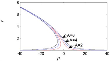
Since the system natural frequency is changed in essence when parameter $p$ is detuned in Eq. (6), the nonlinear characteristic of the system can be revealed through the relationship between the $r$ and $p$. In Eq. (18), when the parameters are $\epsilon =\text{1}$, $\alpha =\text{1}$, $\omega =\text{1}$, $\delta =\text{0.5}$, $A=\text{2,}\text{4,}\text{6}$. The amplitude-frequency curve is obtained as shown in Fig. 2. In this figure, the tongue structure is observed obviously, and the resonant frequency shift phenomenon is exhibited. The advantage for the nonlinear vibration isolation system is to avoid the large vibration amplitude at resonance regime.

2.3. Global dynamic behavior characteristic of the system

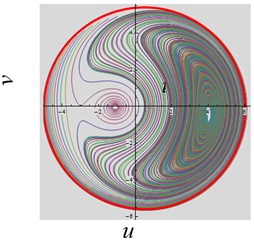
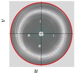
The global dynamic behavior characteristic of the system can be analyzed on the Vander Pol plane, and reveals its long-term trend. The advantage of this method is to avoid the infinite time numerical analysis to judge whether the system terminal behavior is stable or instable. Specially, when the parameters are close to the tongue area, the phase space flow moves at slow speed, but the trajectory will be increased in secular when time approaches infinity. Secondly, the system behavior can be controlled through the parameters based on the Van der Pol plane. Three cases are disused in detail as follows:

(1) The parameter $\gamma$ is varied. When the parameters $\xi =\text{0.1}$, $\gamma =-1$, $f=\text{10}$, $\tilde{\omega }=\text{3}$, system approaches to a stable periodic state, as shown in Fig. 3(a). When $\gamma$ is change to –6, the basic property of the dynamics is invariant except for the trajectories on the left-hand side of the plane become denser, as shown in Fig. 3(b).

Fig. 3The convergent dynamical characteristic of the system when parameter γ is varied

a)

b)

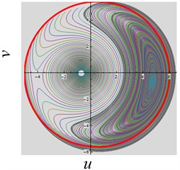
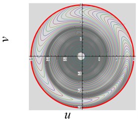
Fig. 4The convergent dynamical characteristic of the system when parameter f is varied

a)

b)

(2) The excitation amplitude parameter $f$ is varied. When the parameters $\xi =$0.1, $\gamma =$ –1, $f=$ 3, $\tilde{\omega }=$ 3 and the parameter $f$ is decreased from 10 to 3, the dynamic behavior still approaches to two stable state, as shown in Fig. 4(a). But when the $f=\text{0.3}$, it is interesting that the system approaches to one stable regime only, as shown in Fig. 4(b), which means that the system oscillates in one potential well.

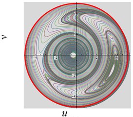
(3) The excitation frequency parameter $\tilde{\omega }$ is varied. When $\xi =\text{0.1}$, $\gamma =-\text{1}$, $f=\text{0.4}$, $\tilde{\omega }=\text{2}$ and the frequency is decreased from 3 to 2, and system works in a periodic state and approaches to one stable regime, as shown in Fig. 5(a). When the $f$ is varied from 0.4 to 1, the system approaches to two stable domains, as shown in Fig. 5(b).

Fig. 5The convergent dynamical characteristic of the system when parameter ω~ is varied

a)

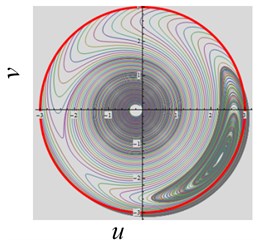
b)

2.4. Lyapunov exponent curve analysis

For system (1), the Lyapunov exponent spectrum combined with the bifurcation analysis is an effective way to judge whether the system works in a chaotic or not. If the Lyapunov is positive, the system works in a chaotic state. When the parameters are $\xi =\text{0.1}$, $\tilde{\omega }=\text{3}$, $\gamma =$ –1, and the excitation force amplitude $f$ is varied from 0.1 to 10, the bifurcation diagram is obtained in Fig. 6.

In Fig. 6, there are abundant dynamical behaviors being revealed. When the excitation force amplitude $f$ is small, the system exhibits period-1 response, and the double-period bifurcation happens at the $f$ is 0.8. The multiple periodic motion and chaos interleave in the range from 2 to 5. In order to identify the chaos parameter regime precisely, the Lyapunov exponent spectrum is calculated, as shown in Fig. 7.

Fig. 6The global bifurcation of the system with the variation of f

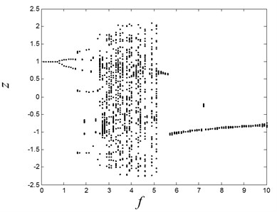
Fig. 7The Lyapunov exponent spectrum with the variation of the f

In this figure, the chaos parameters can be determined on the abscissa axis. Some cases are selected to discover the different dynamic characteristics of the system. When $f$ is 0.1, the system exhibits period-1 motion, the Poincaré section is one point on the phase plane, and the limit cycle is observed, as shown in Fig. 8(a).

When $f$ is 3.4, the system works in a chaotic state, and the strange attractor is given as shown in Fig. 8(b). The corresponding Lypunov exponent is 0.035, and it is positive one, which is the index for chaos. When the $f$ is increase to 3.5, the period-2 motion is presented, and two Poincaré section points lie on the phase plot, as shown in Fig. 8(c). When the $f$ is increase to 4.4, the system comes back to chaos again, as shown in Fig. 8(d).

In order to verify that the calculation is accurate, the Lyapunov exponent spectrum characteristic is checked. The system (1) is rewritten as the following form:

19

$\left\{\begin{array}{l}{\dot{z}}_1=z_2,\\ {\dot{z}}_2=-\xi z_2-\gamma z_1-\beta {z_1}^3+f\mathrm{c}\mathrm{o}\mathrm{s}{z}_3,\\ {\dot{z}}_3=\tilde{\omega }.\end{array}\right.$

Fig. 8The different response phase plane diagram when the parameter f is varied

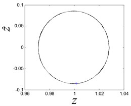
a) The limit cycle when $f$ is 0.1

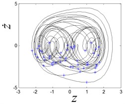
b) Chaotic response when $f$ is 3.4

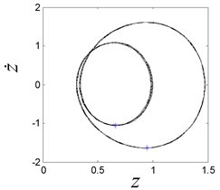
c) The period-2 response when $f$ is 3.5

d) Chaotic response when $f$ is 4.4

According to the phase space flow evolution, the divergence of $f$ is get:

$div\left(f\right)=\frac{\partial f_1}{\partial z_1}+\frac{\partial f_2}{\partial z_2}+\frac{\partial f_3}{\partial z_3}=-\xi ,$

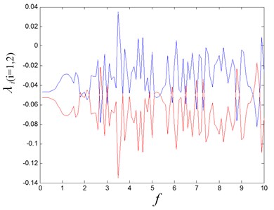
where $f=(f_1,f_2,f_3{)}^T$ is composed of right hand side components of Eq. (19). Thus, the initial phase space volume $V\left(0\right)$ will converge in the form of $V\left(t\right)=V\left(0\right)e^{-\xi t}$. In essence, it is also considered as that the volume converges in the different phase space directions with the law of $V\left(t\right)=V\left(0\right)e^{({\lambda }_1+{\lambda }_2+{\lambda }_3)t}\text{.}$ Therefore, the Lyapunov exponent spectrum ${\lambda }_i$$\text{(}i=$1, 2, 3) characterizes the convergent behavior of the system, and it satisfied with $\sum _{i=1}^3{\lambda }_i=-\xi$. As an example, parts of Lyapunov exponents are listed in table1. Because ${\dot{z}}_3$ keeps constant, the Lyapunov exponent ${\lambda }_3$ is 0. The summation of the other two exponents is –0.1. It meets the elationship between Lyapunov exponent spectrum and damping coefficient.

Table 1Lyapunov spectrum when the excitation amplitude f is varied from 0.5 to 0.8

Excitation amplitude	0.5	0.6	0.7	0.8
Lyapunov exponent ${\lambda }_1$	–0.0462	–0.0451	–0.0436	–0.0393
Lyapunov exponent ${\lambda }_2$	–0.0538	–0.0549	–0.0564	–0.0607

When the excitation amplitude is fixed to 4.4, and the parameter $\tilde{\omega }$ is increased from 0.1 to 10, the global bifurcation diagram is obtained, as shown in Fig. 9. The chaotic vibration occurs in the low frequency regime, and the multi-periodic motion exhibits in high frequency regime. Therefore, in the experiment, the excitation frequency should be adjusted to low frequency range to observe chaos.

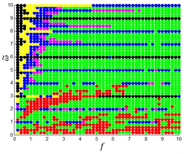
In order to get the global dynamics of the system, the comprehensive response characteristic diagram is computed under different excitation force and frequency, as shown in Fig. 10. The black is period-1 motion; the yellow is period-2 motion; the blue is period-3 motion, the magenta is period-4 motion; the red is chaotic motion, and the green is the other kinds of multiple-period motions. Seen from the figure, the chaotic behavior occurs close to the system’s natural frequency, 3rd sup-harmonic, and half harmonic frequencies regime.

Fig. 9the different response when the parameter ω~ is varied

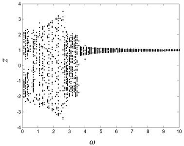
Fig. 10The global comprehensive response of the system when the parameters f and ω~ are varied

3. Finite element analysis of leaf spring

A finite element model (FE) was then used to numerically investigate the natural frequency and vibration mode of the leaf spring system.

Geometrical parameters and material properties of the leaf spring system are shown in Tables 2 and 3. The excitation, a longitudinal force and a transversal disturbance with 30 % strength of the longitudinal force, was applied at one end of the leaf spring (with the other end restricted). Details of excitation are shown in Table 4.

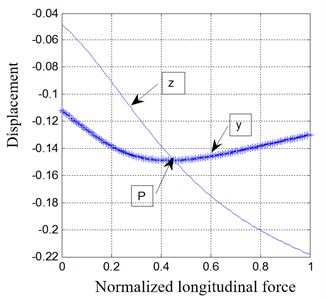
A four-node rectangular element was used with a maximum mesh size of 0.054 mm. The geometry and mesh of the system are shown in Fig. 11. Displacements on $y$ and $z$ directions at the free end of the leaf spring are shown in Fig. 12, against the value of normalized longitudinal force.

From Fig. 12, the displacement in the $y$ direction is a concave curve, which indicates a nonlinear buckling and two possible positions on the curve nearby the point $P$. This means the system can potentially cause chaotic states.

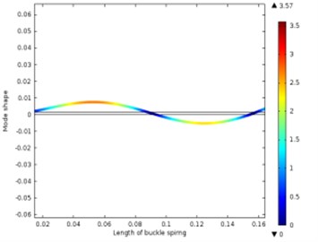
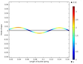
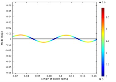
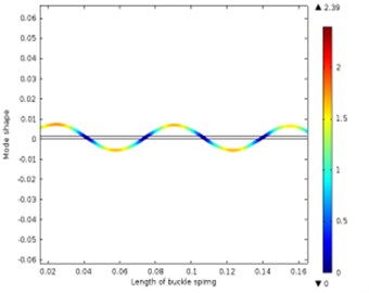
When the leaf spring is installed as a cantilever, the first 6 order natural frequencies obtained from the FE model are shown in Table 5, and the relevant vibration modes are shown in Fig. 13.

Fig. 11Geometry and mesh of the leaf spring system

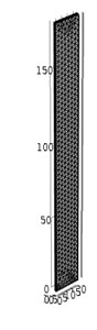
Fig. 12Displacement of the leaf spring in y and z direction

To drive the system entering chaotic vibration regime, the excitation frequency should be close to the system’s natural frequency or its harmonic/half harmonic frequencies. Since the system’s first order natural frequency is 26.664 Hz, the excitation frequency ranges in later experimental study will be focused on the range from 5 Hz to 27 Hz which covers the first order natural frequency and its half harmonics.

4. Test rig set-up

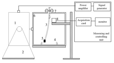
The test rig was designed based on the double potential well principle. As seen in Fig. 14(a).

It has 8 major components, including:

1) Exciter (JZK-50) which provides single frequency excitation to the external frame. Frequency of the excitation was controlled by signal generator (YE1311). Strength of the excitation was controlled by power amplifier (YE5872A);

2) Support base which is used to keep the exciter in a horizontal state;

3) Leaf spring which has the same geometry and material properties as shown in Tables 2 and 3;

4) Rectangular magnet which is used to produce external force;

5) Iron tip which is a small piece of iron. It was placed on the tip of the leaf spring and can be attracted by the magnets;

6) External frame which is used to install magnets and connect exciter;

7) Clamp which is used to fix the end of leaf spring;

8) Laser vibrometer (OPTEX CD33-30NV) which is used to measure the displacement of the leaf spring. It can measure maximum displacement of ±4 mm, with a maximum error of ±0.1 % F.S. Distance between the vibrometer and the leaf spring is 30 mm. The laser vibrometer is connected to a data acquisition card (NI4472).

Fig. 13Different vibration modes of the leaf spring

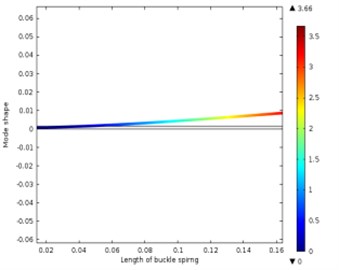
a) The first-order vibration shape

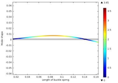
b) The second-order vibration shape

c) The third-order vibration shape

d) The fourth-order vibration shape

e) The fifth-order vibration shape

f) The sixth-order vibration shape

LabVIEW was used to control the DAQ card and online monitor the time history and frequency spectrum. During the experiment, the vibration signal was recorded by the DAQ card with a sampling rate of 2 kHz and a total record time of 5 s for each record. The excitation frequency was adjusted from 5 Hz to 27 Hz with a step of 0.1 Hz. Measurement was repeated under each frequency. Recorded signals were analysed in both time domain and frequency domain. Characteristic frequencies were identified from the frequency spectrum. After phase space reconstruction, the characteristic exponents of the measured signals were obtained with the nonlinear time series analysis method. The chaos identification code was programmed using newly developed signal processing techniques, including improved LE exponent [33] Poincaré section [34], and Wavelet-SG-EEMD, which will be discussed in Section 5.

5. Wavelet-SG-EEMD denoising model

In experiment, recorded chaotic vibration signals are always contaminated by noise from background, electronics and local disturbances. Since the chaotic vibration signals are non-stationary and nonlinear, traditional linear filtering methods are not effective. Therefore, a new combined denoising model is used here. This model uses a Wavelet-SG algorithm which was developed based on the wavelet transform [30] and Savitzky-Golay (SG) theory [32] as pre-filter, and used Ensemble Empirical Mode Decomposition(EEMD) [31] method to reduce the noise and local disturbances.

Fig. 14Leaf spring chaotic vibration experimental rig. 1. Shaker; 2. Support base; 3. Leaf spring; 4. Magnet; 5. Iron tip; 6. External frame; 7. Clamp; 8. Laser vibrometer

a) Sketch of the experimental rig

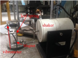
b) Photo of the experimental rig

Fig. 15Flow chart of denoising procedure of Wavelet-SG-EEMD method

The signal processing flow chart of using this Wavelet-SG-EEMD denoising model is shown in Fig. 15, and the detailed procedures are as follows.

Obtain the signal’s wavelet coefficients of each scale by applying wavelet decomposition:

where $c_{j,k}$ and $d_{j,k}$ are approximated coefficients and detailed coefficients respectively, $h$ and $g$ are impulse responses of the filter, and $j$ is the decomposition level of the response.

Reduce the noise using SG method which is presented in Eq. (21). When $s_i$ is one of the IMF (Intrinsic Mode Function) coefficients, a polynomial $p\left(s_i\right)$ with $M$ the order is fitted by $n_l+n_r+$1 points in the vicinity of $s_i$, among which $n_l$ is the number of the left point of $s_i$, and $n_r$ is the number of the right point of $s_i$. The smooth value $q_i$is:

where $\mathrm{\Delta }s=s_{i+1}-s_i$; $b_k$ is the coefficient of $p\left(s_i\right)$. Suppose the measurement data is $y_i$, in order to fit the testing data with $p\left(s_i\right)$, the coefficient $b_k$is determined by optimized function:

Keep the wavelet coefficients in low frequency band unchanged, process the detailed wavelet coefficients with Eq. (23):

where the $T_j$ is the threshold at the $j$th level of wavelet decomposition. Because the variance and the amplitude of the noise will decrease with the increase of the decomposition level, a variable threshold is set as $T_j=\sigma \sqrt{2\mathrm{l}\mathrm{o}\mathrm{g}n}/\sqrt{j+1}$ depending on the variance $\sigma$ of noise, data length $n$ and the decomposition level $j$, and thus details of the useful signals are preserved as much as possible.

Reconstruct signal with the approximated and detailed coefficients with wavelet reconstruction algorithm Eq. (24):

Add random white noise $n_i\left(t\right)$ to reconstructed signal $x\text{'}\left(t\right)$:

where $i=$1, 2, 3,…, $M$, $M>\text{1}$.

Decompose the signal $x_i\left(t\right)$ into IMFs $a_{ij}\left(t\right)$ ($j=$1,…, $N$) through the EMD (Empirical Mode Decomposition), where $a_{ij}\left(t\right)$ denotes the $i$th IMF of the $j$th sample, and $N$ is the number of IMFs. If $j<M$ then go to the step (5) with $j=j+1$. Repeat steps (5) and (6) with different white noise time series at each time.

Finally, calculate the ensemble average $a_j\left(t\right)$ of the $M$ samples for IMF, and reconstruct the original signal:

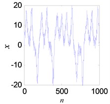
A noisy Lorenz time series is used to test performance of the proposed denoising model. The $SNR$ of Lorenz is set to 5 dB, and the length is 1000. As shown in Figs. 16(a), (b), the proposed denoising model can significantly reduce the noise from chaotic signal. The measured signal of experiment is processed in Figs. 16(c), (d).

Fig. 16The denoising result of Wavelet-SG-EEMD method

a) The noisy Lorenz time series

b) The denoising result

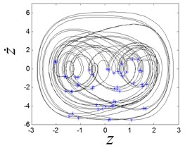
c) Reconstructed attractor on phase plane with original measured signal

d) Reconstructed attractor on phase plane with denoised signal

6. Experimental results analysis and discussion

6.1. Vibration responses under different strength of excitation.

The excitation frequencies studied in the experiment are from 5 Hz to 27 Hz and the output voltage of power amplifier (OVA)is up to1.5 V. The frequency was adjusted with a step of 0.1 Hz. The output voltage of power amplifier was then adjusted from 0 to 1.5 V under each frequency step.

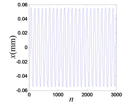
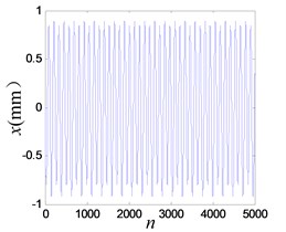
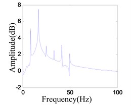
The iron tip falls into the right potential well and oscillates in a period-1 mode (a limit cycle in phase space), when the excitation frequency is 15.6 Hz and output voltage of amplifiers 0.1 V. As shown in Fig. 17(a), the amplitude of the vibration is 0.056 mm. Fundamental frequency (15.6 Hz) and third harmonics (46.8 Hz) are observed, in Fig. 17(b). The reconstruction attractor is a limit cycle, as seen in Fig. 17(c). If a minor disturbance is added to the system, it can be observed from the experiment that the iron tip jumps out of the well and vibrates between two wells. It falls into the left potential well and works in a periodic state after a while, which indicated that the external excitation is not enough to push it out of the well barrier and it is constrained in the potential well fully.

When the excitation is 15.6 Hz and the output of power amplifier is increased to 0.5 V, the vibration amplitude increased to 0.1721 mm. The system shows similar responds, as shown in Fig. 18.

Fig. 17Vibration response when system OVA is 0.1 V

a) Time history of the response

b) Frequency spectrum of the response

c) Reconstructed periodic-1 attractor

d) Poincaré section on limit cycle

Fig. 18Vibration response when system OVA is 0.5 V

a) Time history of the response

b) Frequency spectrum of the response

c) Reconstructed period-1 attractor

d) Poincaré section of cycle

The limit cycle is reconstructed and an improved Poincaré section algorithm is applied to analyze the signal as shown in Fig. 18(c). In order to identify the chaos and periodic mode accurately, at least one point must be located on the limit cycle. However due to the uncertainty from experimentation, the location of the point in the limit cycle may vary slightly. As a result, a number of points are searched in the potential regime as shown in Fig. 18(d) using modified Poincaré method [34].

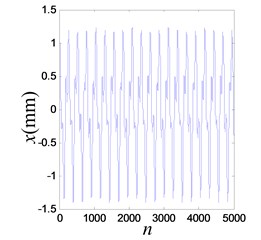
Increasing the output of power amplifier to 0.8 V, the system reaches a critical state where after the same minor disturbance is applied, the system enters chaotic vibration mode which shows that the iron tip jumps between left and right wells randomly. However, the system can still return back to period-1 where the iron tip stays in one of the wells without any disturbance.

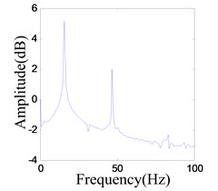
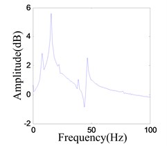
When the output voltage of power amplifier exceeds the critical level, reaches 0.95 V, half harmonics (7.83 Hz) can be recognized Fig. 19(b). This indicates that the doubling periodic is happening in the system.

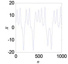
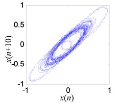
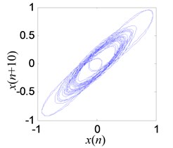
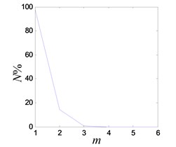
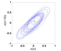
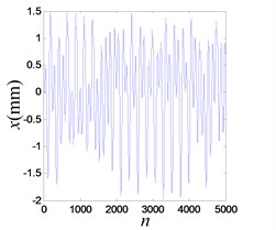
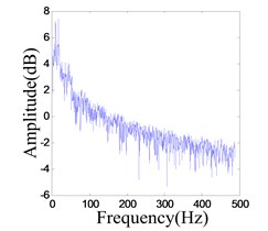
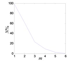
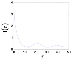
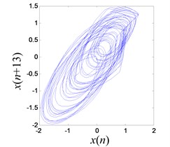
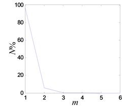
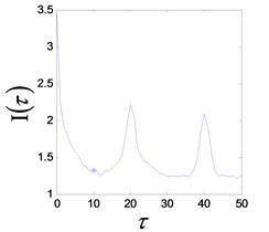
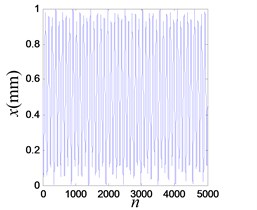
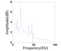
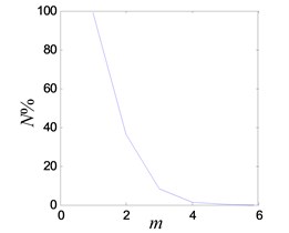
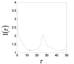
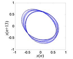
The system enters into a stable chaotic state automatically even without any external disturbance when the output of power amplifier reaches 0.98 V. As shown in Fig. 20(a), the time history is random-like motion and the power spectrum is broadband. The reconstructed phase space parameters are calculated with FNN (false nearest neighbors) and FMMI (first minimum mutual information) methods. The embedding dimension and delay parameters are 4 and 16 respectively, as shown in Figs. 20(c), (d). The chaotic attractor is obtained in Fig. 20(e), and the maximal LE [33] is 0.313.

Fig. 19Vibration response when system OVA is 0.8 V

a) Time history of the response

b) Time history of the response

Fig. 20Vibration response when system OVA is 0.98 V

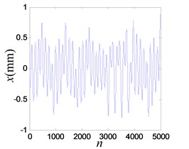
a) Time history of the response

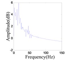
b) Frequency spectrum of the response

c) FNN embedding dimension

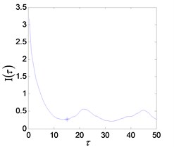
d) FMI reconstruction delay

e) Reconstructed chaotic attractor of system

6.2. Vibration responses under different excitation frequencies

When the output of the power amplifier was less than 0.5 V, changing the excitation frequency from 10 Hz to 17 Hz, the system responses in all the cases stay at period-1 mode. However, when the output voltage of the power amplifier was changed to 1.0 V, the system shows much more complicated responses when frequency varies.

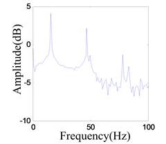
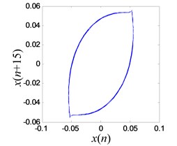
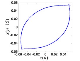
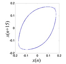
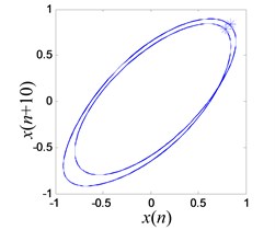
It works in chaotic pattern when the excitation frequencies are in the range of 10 Hz-16 Hz and 17 Hz-19 Hz. When the frequency is 13.4 Hz and system OVA is 1.0 V, the chaotic response is shown in Fig. 21.

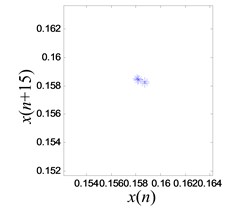
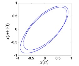
However, there is a certain range, between 16.1 and 16.9 Hz, (e.g. 16.6 Hz), where it works in period-2 mode as shown in Fig. 22, and the LE is –0.0085.

Fig. 21Chaotic vibration response of the system

a) Time history of the response

b) Frequency spectrum of the response

c) FNN embedding dimension

d) FMI reconstruction delay

e) Reconstructed chaotic attractor of system

Fig. 22Period-2 vibration response of the system

a) Time history of the response

b) Frequency spectrum of the response

c) FNN embedding dimension

d) FMI reconstruction delay time

e) Reconstructed period-2 attractor

f) Poincaré section on limit cycle

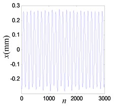
If the frequency is further increased continuously, the system state is changed from chaos to periodic motion. At 19 Hz, the period-3 motion occurs Fig. 23.

Furthermore, when the excitation frequency varied from 19 Hz to 23 Hz, large amplitude multiple periodical vibration between two magnets were observed. This means the iron tip can jump over the potential well peak under these frequencies.

At 23.0 Hz, the multi-periodic motion between double potential wells is shown in Fig. 24 and the vibration amplitude is increased to 1.257 mm.

Fig. 23Period-3 vibration response of the system

a) Time history of the response

b) Frequency spectrum of the response

c) FNN embedding dimension

d) FMI reconstruction delay time

e) Reconstructed period-3 attractor

Fig. 24Multi-periodic vibration response between double potential wells

a) Time history of the response

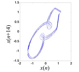
b) Reconstructed multi-periodic attractor

7. Conclusions

A theoretical and experimental study was carried out to investigate the chaotic vibration characteristics of a double potential well leaf spring and magnet system. The nonlinear amplitude frequency characteristic curve is obtained with averaging method [35], and the Lyapunov exponent spectrum combined with the global bifurcation diagram is applied to determine the chaotic regime of the system. A test rig was designed based on the double potential well theory to generate stable and repeatable chaos. The relationship between excitation (strength and frequency) and the leaf system’s nonlinear status was carefully studied. During the experiment, sub-harmonic phenomenon which is an indication of chaos was identified. Some interesting dynamic behaviors occurred, including the two patterns of period-1 motion: one is oscillation in any of the unilateral potential wells; the other is vibration between two wells. The critical state seems to be very sensitive to the excitation. The range of excitation amplitude and frequency where stable and repeatable chaos can be generated were obtained. The signal processing methods, Wavelet-SG-EEMD denoising algorithm and improved Poincaré section method were tested and proved to be effective in identifying chaotic behavior from the system.