Nonlinear dynamic analysis of constant-speed and variable-speed of autonomous vehicle passing uneven road

Yang, Zhiyong; Wang, Long; Liu, Fangtao; Li, Zijian

doi:10.21595/jve.2022.22250

Journal of Vibroengineering

Browse Journal

Submit article

Published: 30 June 2022

Check for updates

Nonlinear dynamic analysis of constant-speed and variable-speed of autonomous vehicle passing uneven road

Zhiyong Yang¹

Long Wang²

Fangtao Liu³

Zijian Li⁴

^{1, 2, 4}College of Computer and Information Science, Chongqing Normal University, Chongqing, P. R. China

^{3, 1}College of Big Data and Internet of Things, Chongqing Vocational Institute of Engineering, Chongqing, P. R. China

Corresponding Author:

Zhiyong Yang

Cite the article Download PDF

Downloads 537

WoS Core Citations 4

CrossRef Citations 2

Abstract

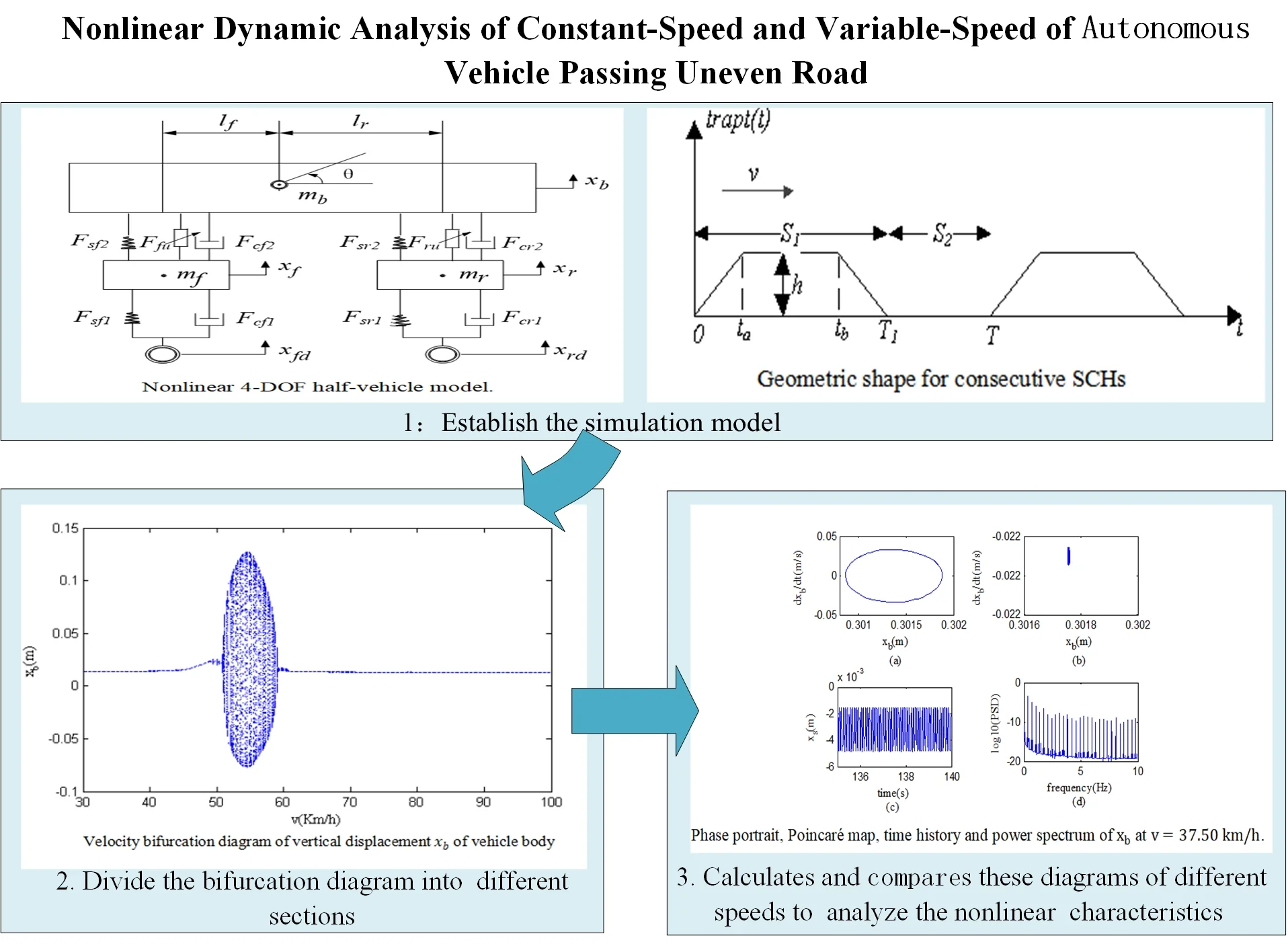
This paper focuses on the research about the comfort and safety of autonomous vehicles passing consecutive speed control humps (SCHs) at a highway, compares and analyzes the nonlinear dynamic characteristics of vehicles driving on uneven roads at a constant speed or with accelerations or decelerations. Firstly, a speed coupling excitation model of the consecutive SCHs and a four-degree-of-freedom (4-DOF) nonlinear vehicle suspension model are established, and then the numerical simulation is carried out by using the four-order fixed-step Runge-Kutta algorithm. The nonlinear dynamic characteristics are analyzed by means of a bifurcation diagram, phase portrait, Poincaré map, time history and power spectrum. Through the analysis, the relevant nonlinear motion characteristics and the speed critical conditions of chaotic vibration of autonomous vehicle suspension under these three conditions are obtained. The results show that chaotic motion may occur when the vehicle passes the uneven road in all three cases, and motion is not periodic during acceleration. Therefore, the vehicle should not accelerate passing continuous SCHs. The experimental results provide support for the follow-up researches of autonomous vehicle, because they give information on how to avoid chaotic motion, speed adaptive control, driving comfort and driving safety.

Nonlinear dynamic analysis of constant-speed and variable-speed of autonomous vehicle passing uneven road

Highlights

When the vehicle moves on the uneven road at a constant speed, the chaotic motion will be caused by the rupture of the quasi periodic ring, and its nonlinear motion law is: periodic motion → quasi-periodic motion → chaotic motion.
When the vehicle decelerates when moving on the uneven road, its law is: chaotic motion →transition state → quasi-periodic motion → periodic motion.
When the vehicle accelerates when moving on the uneven road, the law is: chaotic motion → quasi-periodic motion → chaotic motion.
Chaotic motion may occur when the vehicle both at a constant speed and variable speed moves on uneven roads, and there are similar critical speeds.
Periodic movement will occur when decelerating through uneven road surface, but not when accelerating, so it is inappropriate to accelerate on the uneven road surface.

1. Introduction

With the all-round development of artificial intellect, the automatic driving technology has become one of the latest development trend of the global automobile industry, and vehicle comfort and safety have also become an important research topic of automatic driving technology. According to the relevant research, the automobile suspension system is an important part of automobile, which helps to improve the safety and comfort of automobile. Nowadays, the automotive suspension system contains a large number of nonlinear components, including variable stiffness spring, electro-rheological (ER) damper and magnetorheological (MR) dampers. Complex dynamic characteristics, including chaos and bifurcation [1, 2], will be reflected in the vehicle suspension system running on uneven roads. Chaotic vibration will not only adversely affect the comfort of passengers, but also cause a certain damage to the vehicle itself and the road [3]. For example, Javad Fakhraei and his coauthors simulated the excitation of the continuous SCHs with half-sine wave, studied the chaotic vibration analysis of heavy articulated vehicle (HAV), and proved that the chaotic behavior will directly affect the driving comfort and reduce the riding comfort [4]. Current research demonstrated that one of the factors that had an important impact on vehicle amplitude and vibration intensity was the vehicle suspension system [2, 5, 6]. Under extreme and severe conditions, severe vehicle vibration may damage the suspension system and pose a hazard of rollover and personal injury [7, 8]. However, it can be found that at first most of the initial research on chaotic vibration under road excitation focused on single-degree-of-freedom and two-degree-of-freedom vehicle models, such as the relevant paper of Q. Zhu and his coauthors who used the numerical simulation method to analyze the chaotic vibration of nonlinear two-degree-of-freedom air spring, which opened the way to analyze its influence on the chaotic characteristics of vehicle suspension system from the perspective of road excitation frequency [9]. These excitations include sine wave excitation and multi-frequency, multi-amplitude or random excitation. As a relatively simple vehicle model, single-degree-of-freedom and two-degree-of-freedom vehicle models only study the vehicle movement in the vertical direction, which often cannot reflect the overall dynamic characteristics of the vehicle, and have obvious limitations. It was found that the single-degree-of-freedom and two-degree-of-freedom models could not provide enough information to reflect the actual motion characteristics of the vehicle. The 4-DOF half vehicle model is relatively closer to the actual vehicle model [10]; The model can both reflect the vertical motion and pitch motion of the vehicle body, and demonstrate the vertical motion of front and rear wheels. For example, in order to control the vibration of the wheel hub motor suspension coupling system of electric vehicle as a whole, Wei Wang and his coauthors established a nonlinear dynamic model of a four-degree-of-freedom coupling system composed of motor magnetic gap (MMG), and carried out numerical simulation with MATLAB, so as to search the optimal parameter combination in the nonlinear dynamic model and significantly improve the ride comfort of electric wheel vehicle [11].

At present, when the nonlinear dynamic characteristics of vehicles passing uneven roads are studied, a fixed assumption is often made as follows: vehicles pass uneven roads at a fixed speed, and when the characteristics of nonlinear vehicles passing continuous SCHs through simulation are analyzed, it is assumed that vehicles pass at a constant speed [12]. In reality, the speed of vehicles is not often fixed. It is affected by weather conditions, time and driver’s emotional state. These acceleration or deceleration conditions may also cause vehicle vibration. Maintaining a constant speed or accelerating/decelerating on the road will also lead to non-stationary vibration of the vehicle. In actual road conditions, there are many situations that lead to vehicle vibration, such as: (1) The vehicle runs on a spatially uniform undulating road with a variable speed. (2) The vehicle moves on the uneven road at a fixed speed or variable speed. (3) The vehicle runs on a flat road, then suddenly encounters an uneven road with uniform space, and continues to drive at a fixed speed. In order to facilitate the research, taking the continuous SCHs as the representative of uneven pavement, the conventional continuous speed is transformed into discrete speed by the data fitting method, and the speed change is divided into uniform speed, acceleration and deceleration. It is of great practical significance to study the nonlinear dynamic characteristics of vehicles moving at a constant or variable speed on the uneven road. So, the nonlinear dynamic phenomena of vehicle uniform speed, acceleration and deceleration under the action of the continuous SCHs in automatic driving scene are studied in this paper. The possibility of nonlinear chaotic vibration of vehicle under three modes and the nonlinear motion law of vehicle suspension system are analyzed by the numerical simulation method. Through the research, the critical conditions of chaos and the generation path of chaos in the system are obtained for the period when the vehicle passes the continuous SCHs, and the nonlinear dynamic characteristics of constant speed, acceleration and deceleration are compared and analyzed. The research results lay a foundation for self-adaptive speed regulation, the continuous SCHs design and improves the occupant comfort.

2. Simulation model description

2.1. Nonlinear 4-DOF half-vehicle model

In the 4-DOF half car model, the vehicle can be regarded as a completely symmetrical mechanical structure. Considering the mechanical structure of the front and rear wheels of the suspension system, the four degrees of freedom studied here consider front and rear wheel deformation, 1/2 body vertical vibration and body pitching, and the nonlinearity of front and rear wheels, front and rear suspension springs and suspension dampers. The longitudinal view in Fig. 1 [10, 12] contains a simplified model of 4-DOF half-vehicle. And unsprung mass, spring, suspension and tire are the main parts of the active suspension model. The static equilibrium position here is used as the origin for heave displacements of both front and rear unsprung mass, $x_{f} (t)$ and $x_{r} (t)$ , and also for both angular displacement of the vehicle body mass $θ (t)$ and heave displacement $x_{b} (t)$ .

Fig. 1Nonlinear 4-DOF half-vehicle model

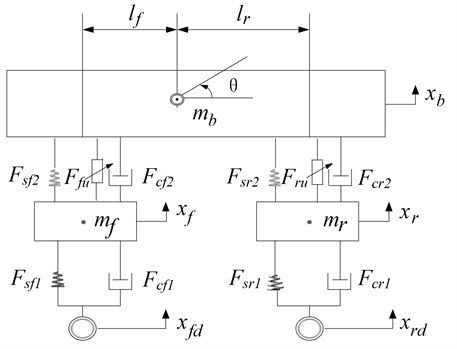
Table 1 lists the symbolic description of the model.

Table 1Model symbol description

Symbol	Symbol description	Symbol	Symbol description
$m_{b}$	Sprung mass	$θ$	Angular displacement of $m_{b}$
$m_{f}$	Front unsprung masses	$m_{r}$	Rear unsprung masses
$l_{f}$	Front lengths	$l_{r}$	Rear lengths
$x_{f d}$	Excitations to the front tire	$x_{r d}$	Excitations to the rear tire
$x_{b}$	Displacements of $m_{b}$	$x_{f}$	Displacements of $m_{f}$
$x_{r}$	Displacements of $m_{r}$	$F_{s f 1}$	Front nonlinear suspension damper forces
$F_{s r 1}$	Rear nonlinear suspension damper forces	$F_{s f 2}$	Front nonlinear suspension spring forces
$F_{s r 2}$	Rear nonlinear suspension spring forces	$F_{c f 2}$	Front suspension damper forces
$F_{c r 2}$	Rear suspension damper forces	$F_{c f 1}$	Front nonlinear tire spring forces
$F_{c r 1}$	Rear nonlinear tire spring forces	$F_{f u}$	Active control forces of rear suspensions
$F_{r u}$	Active control forces of front suspensions	$J$	The moment of inertia of the pitch axis

Based on the second Newton law, the following equations of motion can be made:

1

\{\begin{matrix} m_{b} {\ddot{x}}_{b} = - F_{s f 2} - F_{c f 2} - F_{s r 2} - F_{c r 2} - m_{b} g, \\ J \ddot{θ} = (F_{s f 2} + F_{c f 2}) l_{f} \cos θ - (F_{s r 2} + F_{c r 2}) l_{r} \cos θ, \\ m_{f} {\ddot{x}}_{f} = F_{s f 2} + F_{c f 2} - F_{s f 1} - F_{c f 1} - m_{f} g, \\ m_{r} {\ddot{x}}_{r} = F_{s r 2} + F_{c r 2} - F_{c r 1} - m_{r} g . \end{matrix}

Setting $x_{1} = x_{b}$ , $x_{2} = {\dot{x}}_{b}$ , $x_{3} = θ$ , $x_{4} = \dot{θ}$ , $x_{5} = x_{f}$ , $x_{6} = {\dot{x}}_{f}$ , $x_{7} = x_{r}$ , $x_{8} = {\dot{x}}_{r}$ , the system state equations is as follows:

2

\{\begin{matrix} {\dot{x}}_{1} = x_{2}, \\ {\dot{x}}_{2} = - \frac{1}{m_{b}} (F_{{s f}_{2}} + F_{{c f}_{2}} + F_{{s r}_{2}} + F_{{c r}_{2}}) - g, \\ {\dot{x}}_{3} = x_{4}, \\ {\dot{x}}_{4} = \frac{\cos θ}{J} [(F_{{s f}_{2}} + F_{{c f}_{2}}) l_{f} - {(F}_{{s r}_{2}} + F_{{c r}_{2}} l_{r})] - g, \\ {\dot{x}}_{5} = x_{6}, \\ {\dot{x}}_{6} = - \frac{1}{m_{f}} (F_{{s f}_{2}} + F_{{c f}_{2}} - F_{{s f}_{1}} + F_{{c f}_{1}}) - g, \\ {\dot{x}}_{7} = x_{8}, \\ {\dot{x}}_{8} = - \frac{1}{m_{r}} (F_{{s r}_{2}} + F_{{c r}_{2}} - F_{{s r}_{1}} + F_{{c r}_{1}}) - g . \end{matrix}

2.2. Excitation model of consecutive SCHs

Fig. 2(a) shows the real scene of the consecutive SCHs of an expressway provided for reference. In Fig. 2(b), the continuous trapezoidal wave was developed to approximately simulate the excitation of the consecutive SCHs. S1 is the width of the consecutive SCHs, $h$ is the height of the consecutive SCHs, S2 is the distance of two adjacent bumps. To make the vehicle pass continuous SCHs stably, safely and effectively, the value of $h$ is generally averaged as 1.0 cm ~ 2.0 cm, and the square values are $S_{1}$ = 50 cm~100 cm, $S_{2}$ = 50 cm~100 cm. And $t_{S_{1}} = S_{1} / v$ is the time to pass the consecutive SCHs, $t_{S_{2}} = S_{2} / v$ is the time to move on the gap between two adjacent humps. Thus, the incentive period is $T = t_{S_{1}} + t_{S_{2}}$ , and the relationship between the vehicle speed $v$ and the excitation frequency $f$ can be represented as:

3

f = \frac{1}{T} = \frac{v}{S_{1} + S_{2}} .

The time difference between the front and rear wheels is defined as $∆ t$ , and the front wheel excitation is expressed as follows:

4

x_{f d} = t r a p (t),

where:

5

t r a p (t) = \{\begin{matrix} \frac{h}{t_{a}} \times t, t \leq t_{a}, \\ h, t_{a} < t \leq t_{b}, \\ \frac{h}{T_{1} - t_{b}} \times (T_{1} - t), t_{b} < t \leq T_{1}, \\ 0, T_{1} < t < T . \end{matrix}

The lag relationship between the front wheel and the rear wheel as the time lag between the front wheel driving at a point on the road and the rear wheel passing the same point at the same speed is expressed as follows:

6

Δ t = \frac{l_{f} + l_{r}}{v},

where $l_{f}$ , $l_{r}$ represent the distances between the vehicle center and the front wheels, the rear wheels.

Fig. 2Consecutive SCHs geometric shape

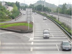
a) SCHs in highway turn section or ramp

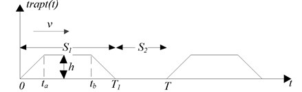
b) Geometric shape for consecutive SCHs

The rear wheel excitation can be expressed as follows:

7

x_{r d} = t r a p (t + Δ t) .

Eqs. (3) and (6) lead to:

8

Δ t = \frac{T (l_{f} + l_{r})}{S_{1} + S_{2}} .

It can be seen from Eq. (8) that the lag of front and rear wheels is related to the length of the vehicle itself and the width and preset distance of bumps.

2.3. Instantaneous speed representation

The instantaneous speed of a vehicle on an uneven road is very important, regardless of whether it is decelerating or accelerating. The empirical mathematical function is introduced for averaging the difference between the system input and output by means of data fitting. In order to ensure that the research data are consistent with the actual situation, the fifth-order fitting mathematical expression is used here, and a group of data is randomly selected within 30 km/h-100 km/h. This fitting expression is as follows:

9

v_{0} = [a_{1} X^{5} + a_{2} X^{4} + a_{3} X^{3} + a_{4} X^{2} + a_{5} X + a_{6}],

where:

10

[\begin{matrix} a_{1} \\ a_{2} \\ a_{3} \\ a_{4} \\ a_{5} \\ a_{6} \end{matrix}] = [\begin{matrix} 4.9084 \times 1 0^{- 7} \\ - 1.4323 \times 1 0^{- 4} \\ 1.55 \times 1 0^{- 2} \\ - 7.583 \times 1 0^{- 1} \\ 1.64461 \times 1 0^{1} \\ - 7.71952 \times 1 0^{- 1} \end{matrix}] .

$a_{1} ~ a_{5}$ are the multinomial coefficients of one to five orders, and $a_{6}$ is the initial fitting speed, $X$ is the fitting step size, and $v_{0}$ is the fitting speed.

2.4. Simulation parameters

Fig. 1 shows the simulation object considered in this paper, and Table 2 shows the model parameters [10]. The static equilibrium parameters are set as the initial conditions of the simulation by $[x_{b}, {\dot{x}}_{b}, θ, \dot{θ}, x_{f}, {\dot{x}}_{f}, x_{r}, {\dot{x}}_{r}] = [0,0, 0,0, 0,0, 0,0]$ , and the step size is set to 0.02 km/h. The four-order fixed step Runge-Kutta algorithm is used to study the dynamics of vehicle model accurately with the consideration of nonlinearity of differential equations.

Table 2Specific parameters set in numerical simulation

Parameter	Value	Parameter	Value	Parameter	Value
$m_{b}$	1180.0 kg	$J$	633.615 kg.m²	$c_{r 1}$	10 kg/s
$m_{f}$	50.0 kg	$l_{f}$	1.123 m	$c_{f 2 u}$	500 kg/s
$m_{r}$	45.0 kg	$l_{r}$	1.377 m	$c_{f 2 d}$	359.7 kg/s
$k_{f 1}$	140000.0 N/m	$n_{f 1}$	1.25	$c_{r 2 u}$	500 kg/s
$k_{r 1}$	140000.0 N/m	$n_{r 1}$	1.25	$c_{r 2 d}$	359.7 kg/s
$k_{f 2}$	36952.0 N/m	$n_{f 2}$	1.5	$h$	0.015 m
$k_{r 2}$	30130.0 N/m	$n_{r 2}$	1.5	$s_{1}$	500 mm
$g$	9.81 N/kg	$c_{f 1}$	10 kg/s	$s_{2}$	500 mm

3. Nonlinear feature extraction method

The identification methods of chaos can be divided into three categories: theoretical identification method, experimental method and numerical simulation method. At present, the theoretical chaos analysis method is not mature, especially when it comes to study a relatively complex nonlinear vehicle suspension system with 4-DOF or higher, the theoretical analysis method is not very ideal. Experimental analysis refers to the discovery of chaos from experimental phenomena by establishing a simple system experimental model. Because chaotic vibration has strong initial value sensitivity, the experimental method has high requirements for experimental equipment. The loss, aging and experimental environment of experimental equipment can have a great impact on the experimental results leading to the completely undetermined results. Especially for the relatively complex nonlinear vehicle suspension system, the experimental analysis method is more difficult. Among the methods of chaos identification, numerical simulation is the most extensive and practical method, which usually includes bifurcation diagram, phase portrait, Poincaré map, time history and power spectrum.

Fig. 3Example of bifurcation diagram

3.1. Bifurcation diagram

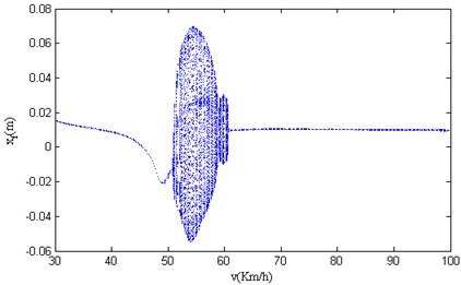
Bifurcation diagram is a graph space composed of state variables and bifurcation parameters, which represents the change of state variables with time. The abscissa of the bifurcation diagram is a continuously changing quantity selected in the system, and the ordinate is the Poincaré section of the system corresponding to the selected quantity. The parameter range corresponding to different motion forms of the system can be obtained through this bifurcation diagram. According to the parameter range, the whole motion region of the system is roughly divided into different single motion forms. As shown in Fig. 3, Bifurcation diagram, the entire speed section is divided into three regions: A (30.00 km/h-46.10 km/h), B (46.10 km/h-61.60 km/h), C (61.60 km/h-100.00 km/h).

3.2. Phase portrait

The system state is made up of the solution vector composed of the solutions of multiple state variables of the system. The space composed of these state variables is called the phase space. The curve depicting the solution of the state equation in the phase space is called the phase trajectory, and these phase trajectories of the state equation constitute the phase diagram. The trajectory of the phase diagram of periodic motion consists of one or more closed curves. The phase trajectories of quasi-periodic motion and chaotic motion are full of phase space and non-repetitive curve sets. The phase diagram in Fig. 4 is composed of multiple closed curves, which can be assessed as quasi-periodic motion or chaotic motion.

Fig. 4Example of phase portrait

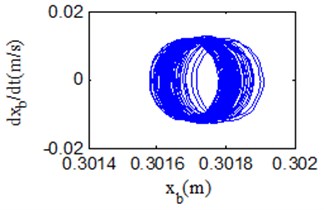
Fig. 5Example of Poincaré map

3.3. Poincaré map

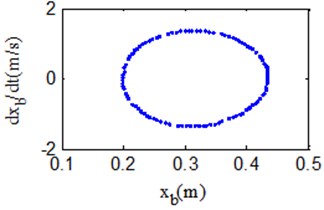
Poincaré diagram discretizes the curve in the phase diagram into phase points, which can be understood as making a vertical section in the phase space plane. When the Poincaré section is a point, the system moves periodically. When there are $n$ points ( $n \geq$ 2) on the Poincaré section, the system makes $n$ -periodic motion. When the obtained Poincaré cross section is a closed ring, the system makes quasi-periodic motion. When it is an infinite set of irregular points, the system is chaotic motion. As shown in Fig. 5, the Poincaré section is presented as a closed loop, which can be assessed as quasi-periodic motion.

3.4. Time history

Time history can clearly reflect the change trend of system response with time, and can qualitatively observe the global characteristics of system response. It is the most intuitive method to observe the chaotic phenomena. The time history of chaotic motion and quasi-periodic motion are continuous, while the corresponding time history of periodic motion is column discrete. As shown in Fig. 6, it is a time history chart, which can be assessed as quasi-periodic motion or chaotic motion.

3.5. Power spectrum

Power spectrum is the result of frequency division statistics of system response. It demonstrates the characteristics of system energy distribution by frequency. Power spectrum is another method to identify the chaotic motion of the system. The time series of periodic motion can be expanded into Fourier series, and the corresponding spectrum is column discrete. The time series of periodic motion can only be expanded into Fourier integral, and the corresponding spectrum is continuous. In addition, the power spectrum can also identify quasi-periodic motion and chaotic motion to a certain extent, but the discrete spectral lines of quasi-periodic motion are dense, seemingly continuous but discrete in nature, and the spectral lines of chaotic motion are completely continuous. As shown in Fig. 7, it is a power spectrum, which is column discrete and can be assessed as periodic motion.

Fig. 6Example of time history

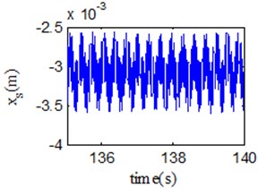
Fig. 7Example of power spectrum

4. Analysis of nonlinear dynamic characteristics of vehicles moving on uneven road surface at constant speed

In this paper, the 4-DOF half-vehicle model shown in Fig. 1 is taken as the simulation object, the periodic trapezoidal wave excitation shown in Fig. 2 is used to simulate the roughness of the speed control bump, and Table 2 is added to describe the simulation model parameters.

Fig. 8Velocity bifurcation diagram of 4-DOF parameters

a) Velocity bifurcation diagram of vertical displacement $x_{b}$ of vehicle body

b) Velocity bifurcation diagram of pitch angle $θ$ of vehicle body

c) Velocity bifurcation diagram of vertical displacement $x_{f}$ of vehicle’s front wheel

d) Velocity bifurcation diagram of vertical displacement $x_{r}$ of vehicle’s rear wheel

This paper applies the four-order fixed step Runge-Kutta algorithm which is available in MATLAB to solve the Eq. (1), and studies the dynamic response of the 4-DOF nonlinear vehicle suspension model under the excitation of periodic consecutive SCHs. The nonlinear characteristics studied in this paper are based on the condition of system stability. Usually, it takes a certain time for the system to change over from initial condition to stable condition, which requires the excitation to last long enough, so the excitation step size cannot be too short. In order to remove the transient response of the system and make the simulation retain the completely steady-state behavior, the simulation step is 0.01 km/h, The velocity bifurcation diagram of the 4-DOF parameters in the paper is shown in Fig. 8.

It can be seen from Fig. 8 that the vibration has changed significantly when the vehicle passes the consecutive SCHs with the speed varying within 30.00 km/h-100.00 km/h, and the vibration becomes complicated when the vehicle speed varies within 46.10 km/h-61.60 km/h, which means that chaotic motion occurs when the velocity is in or near the unstable range. At the same time, the four bifurcation diagrams have similar motion characteristics. Therefore, based on the difference in nonlinear characteristics presented by different speed sections, the entire speed section is divided into three regions: A (30.00 km/h-46.10 km/h), B (46.10 km/h-61.60 km/h), C (61.60 km/h-100.00 km/h).

Due to the unstable region of the system, in order to further reveal the possible chaotic vibration related to the system parameters $x_{b}$ , $θ$ , $x_{f}$ and $x_{r}$ , this paper selects speeds of $v =$ 37.50 km/h, $v =$ 54.20 km/h and $v =$ 67.20 km/h respectively in the regions A, B and C to calculate the phase diagram, Poincaré mapping, time history and power spectral density of the system and we focuses on the nonlinear vibration characteristics of the system under the coupling excitation of periodic the continuous SCHs and periodic pavement. Because the four bifurcation diagrams have similar motion characteristics in the same speed range, the paper only calculates and analyzes the phase diagram, Poincaré mapping, time history and power spectral density at speeds of $v =$ 37.50 km/h, $v =$ 54.20 km/h and $v =$ 67.20 km/h as an example, which is shown in Figs. 9-11.

Fig. 9Phase portrait, Poincaré map, time history and power spectrum of xb at v= 37.50 km/h

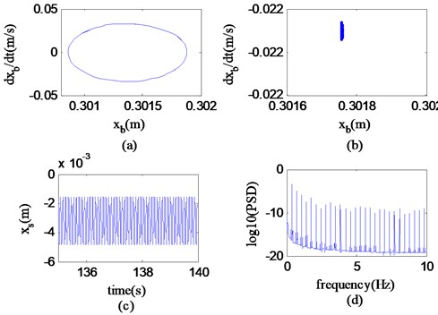
The phase diagram in Fig. 9 is a closed curve. The Poincaré section should be a straight line, and the abscissa and the ordinate contain only certain values (as one point). The time history shows periodic changes. After the logarithm of the power spectrum is taken, the quantity of spectral lines becomes fewer. According to the nonlinear feature extraction method, it can be seen that the system moves periodically within the range of 20.00 km/h $\leq v \leq$ 46.10 km/h.

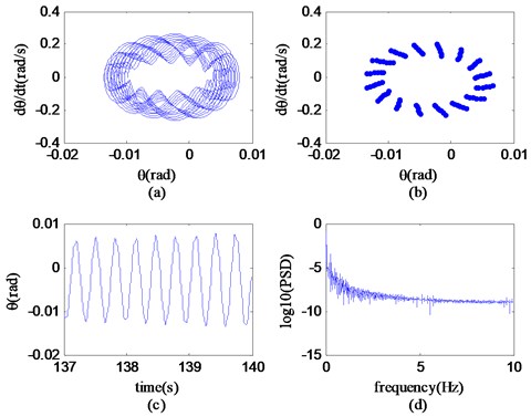
In Fig. 10, the phase diagram has a large number of rings in the form of Hopf rings, the Poincaré section is presented as a closed loop, the time history is generally stable, and the power spectrum is shown as complex spectral lines. According to the nonlinear feature extraction method, it can be inferred that the system makes quasi-periodic motion within the range of 46.10 km/h $\leq v \leq$ 61.60 km/h.

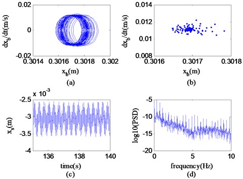
The phase diagram in Fig. 11 is composed of multiple closed curves, which fill the whole phase space. The Poincaré section contains infinite points, the time history changes irregularly, and the logarithmic spectral lines of the power spectrum are distributed in a continuous form. According to the nonlinear feature extraction method, it can be inferred that the system performs chaotic motion within the range of 61.60 km/h $\leq v \leq$ 100.00km/h.

Through the above analysis, the vehicle suspension system is affected by the consecutive SCHs and uneven road surface. With the increase of vehicle speed, the nonlinear motion of the system changes with a law: periodic motion → quasi-periodic motion → chaotic motion. That means the rupture of the quasi-periodic loop leads to the chaotic motion in the system.

Fig. 10Phase portrait, Poincaré map, time history and power spectrum of xb at v= 54.20 km/h

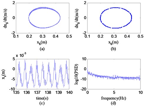
Fig. 11Phase portrait, Poincaré map, time history and power spectrum of xb at v= 67.20 km/h

5. Analysis of nonlinear dynamic characteristics of vehicles moving on uneven road at variable speed

5.1. Analysis of nonlinear dynamic characteristics during vehicle deceleration through consecutive SCHs

The design purpose of continuous SCHs is to prompt or force the driver to slow down and protect the vehicle personnel. This paper assumes that the vehicle enters the continuous SCHs at a speed of 100.00 km/h, and the vehicle speed will change within the speed range of 30.00 km/h-100.00 km/h. In this section, the bifurcation diagram of the system is used to analyze the chaotic vibration characteristics of vehicle deceleration. In order to show the displacement velocity relationship of the vehicle, the bifurcation diagram selects the changing excitation velocity as the abscissa, and the ordinate is the Poincare section of the displacement response of the vehicle with four-degrees-of-freedom parameters [13]. The bifurcation diagram observation and analysis reveal the range of motion in each stage and the corresponding velocity of complex motion. Fig. 12 shows the speed displacement bifurcation diagram of the vehicle.

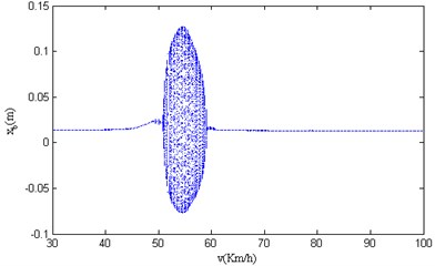
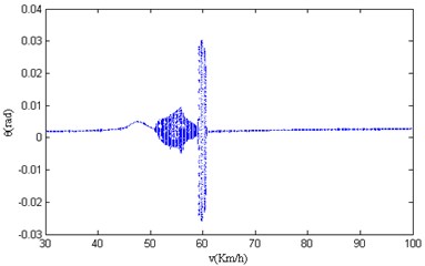
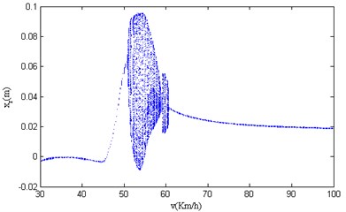
Fig. 12Velocity – displacement bifurcation diagram of 4-DOF parameters of vehicle

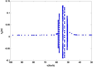
a) Velocity bifurcation diagram of vertical displacement $x_{b}$ of vehicle body

b) Velocity bifurcation diagram of pitch angle $θ$ of vehicle body

c) Velocity bifurcation diagram of vertical displacement $x_{f}$ of vehicle’s front wheel

d) Velocity bifurcation diagram of vertical displacement $x_{r}$ of vehicle’s rear wheel

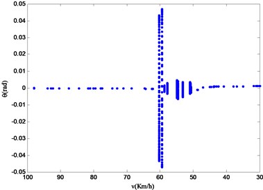
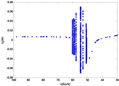
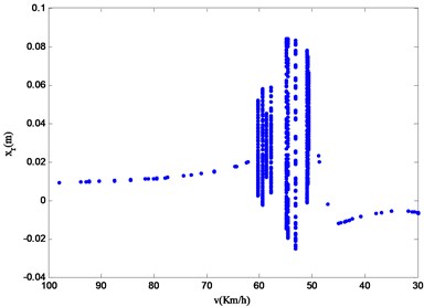
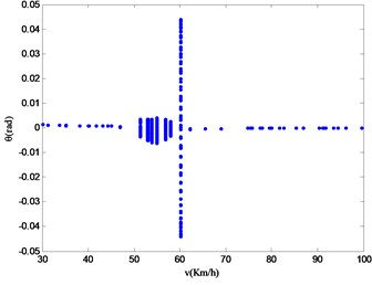
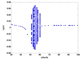
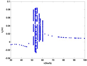
It can be seen from Fig. 12, the four-degrees-of-freedom vehicle speed bifurcation diagram that the system vibration changes obviously within the studied speed range of 100.00 km/h $\geq v \geq$ 30.00 km/h. And the vertical axis values of the velocity bifurcation diagram within the studied speed range are discontinuous and discrete. This means that the vibration amplitude of the vehicle is indeed changing dynamically when the vehicle is running at variable speed, which is not found in the speed bifurcation diagram of the vehicle running at a constant speed in the third part of this paper. At the same time, different system state variables have similar nonlinear characteristics. On the basis of the difference of nonlinear motion characteristics in the bifurcation diagram, the velocity is divided into four regions: region A (100.00 km/h-62.25 km/h), region B (60.28 km/h-59.49 km/h), region C (58.70 km/h-50.79 km/h) and region D (48.68 km/h-30.00 km/h). After the bifurcation diagram is observed, it becomes obvious that the vibration in region B and region C is relatively complex and has the possibility of chaotic vibration.

Fig. 12 is analyzed, and the motion characteristics are compared to find that the state variables $θ$ are significantly different from other variables. So, $θ$ is chosen as the representative for studying the vibration characteristics of the system. Based on the theory of nonlinear vibration, the research and analysis on the specific nonlinear vibration of the system within the range of 100.00 km/h $\geq v \geq$ 30.00 km/h were conducted. Phase diagram, Poincaré section, time history and power spectral density of the vehicle state variable $θ$ , as shown in Fig. 13-16, were plotted after selecting four speeds: 79.48 km/h, 60.28 km/h, 58.70 km/h and 35.07 km/h in the four regions to compare their nonlinear dynamic characteristics.

Fig. 13Phase portrait of θ, Poincaré map, time history and power spectrum at v= 79.48 km/h

It can be seen from Fig. 13 that in the region A (100.00 km/h-62.25 km/h), the trajectory of the state variable $θ$ has multiple closed curves in the phase diagram, Poincaré map has unlimited points, the time history is non-periodic, and the logarithmic spectrum of the power spectrum is continuous. According to the corresponding nonlinear recognition method, it can be known that the state variables $θ$ do chaotic motion at a speed of $v =$ 79.48 km/h. It can be further concluded that the nonlinear motion of the system in the area is chaotic motion.

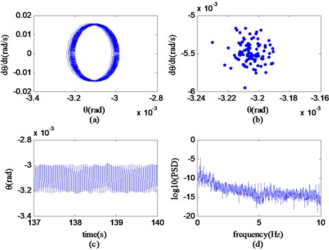
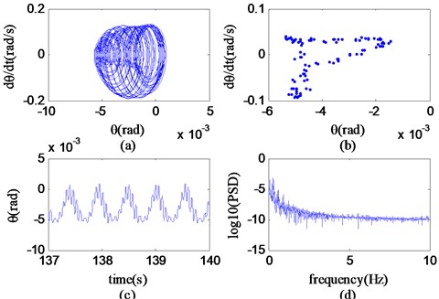
Fig. 14Phase portrait of θ, Poincaré map, time history and power spectrum at v= 60.28 km/h

It can be seen from Fig. 14 that in the region B (60.28 km/h-59.49 km/h), the velocity bifurcation diagram only takes two velocity values, which are respectively 60.28 km/h and 59.49 km/h. The motion trajectory of the state variable $θ$ consists of countless closed and irregular rings in the phase plane; it can be seen that the Poincaré section appears as an incomplete closed loop, the time history graph appears to be relatively stable on the whole, and the power spectrum graph is more complicated. According to the recognition method of corresponding nonlinear characteristics, it can be known that the state variable $θ$ transits from chaotic motion to quasi-periodic motion at a speed of $v =$ 60.28 km/h, which is referred to as the transition state for short. It can be further concluded that the nonlinear motion state of the system in region B is a transition state.

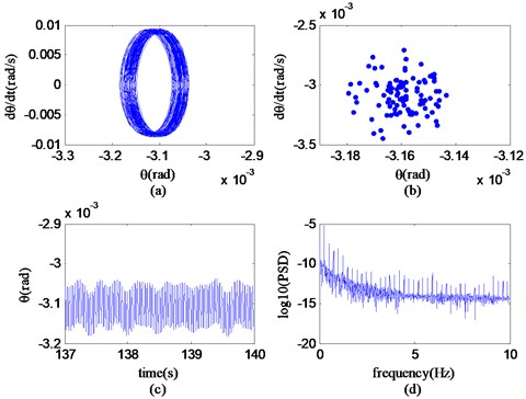
It can be seen from Fig. 15 that in the region C (58.7 km/h-50.79 km/h), the trajectory of the state variable has a form of multiple closed curves in the phase diagram, the Poincaré map is a completely closed loop, the time history is overall stable, and the power spectrum is displayed as discrete spectral lines. According to the recognition method of corresponding nonlinear characteristics, it can be known that the state variable $θ$ moves in a quasi-periodic motion at a speed of $v =$ 58.70 km/h. It can be further concluded that the nonlinear motion of the system in region C is quasi-periodic motion.

Fig. 15Phase portrait of θ, Poincaré map, time history and power spectrum at v= 58.70 km/h

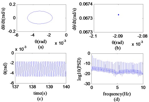
In Fig. 16, within the interval, region D (50.79 km/h-30.00 km/h), the motion trajectory of the state variable $θ$ is a closed loop in the phase diagram, the Poincaré section corresponds to a point, the time history changes periodically, and the power spectrum is logarithmically composed of fewer spectral lines. According to the recognition method of corresponding nonlinear characteristics, it can be known that the state variable $θ$ moves periodically at a speed of $v =$ 35.07 km/h. It can be further concluded that the nonlinear motion of the system in the region D is period-motion.

Through the above analysis, it is revealed that as the vehicle moves on the consecutive SCHs with variable deceleration, affected by combined excitation of consecutive SCHs and uneven road surface, the nonlinear motion law of the vehicle suspension system is chaotic motion → transition state → quasi-periodic motion → periodic motion; the system has the possibility of chaotic vibration, and the critical condition for the chaotic vibration of the system is 60.28 km/h $< v =$ 100 km/h.

In the fourth part of the paper (Section 4), the nonlinear motion law of the vehicle passing the consecutive SCHs at a constant speed is periodic motion → quasi-periodic motion → chaotic motion, while the law of the vehicle variable deceleration through the consecutive SCHs is the chaotic motion → quasi-periodic motion → transition state → periodic motion. By comparison, it is found that the motion laws of the two modes are reversed, and one additional transition exists in the case of variable deceleration. The critical condition of chaotic motion at a constant speed is 100.00 km/h $> v =$ 61.60 km/h, the critical condition for chaotic vibration when passing with the variable deceleration is 60.28 km/h $< v =$ 100.00 km/h, the velocity range of chaotic motion obtained in the two cases is different, but there is the same velocity range of 61.60 km/h-100.00 km/h. The speed range of the periodic motion is 30.00 km/h-46.10 km/h when passing at a constant speed, while the speed range of the periodic motion is 50.79 km/h-30.00 km/h when passing with the variable deceleration. The speed range of the periodic motion obtained in the two cases is different, but there is still the same speed range of 30.00 km/h-46.10 km/h. Through the comparative analysis of the consecutive SCHs, the following conclusions can be drawn:

1) In the two modes, chaotic vibration may occur through consecutive SCHs, and the critical speeds are similar.

2) There are the same periodic motion speed range and chaotic motion speed range when moving on the consecutive SCHs in the two ways, and the speed range when passing with the variable deceleration includes the speed range of passing at a constant speed. Therefore, whether the vehicle passes through the consecutive SCHs at a constant speed or variable deceleration, the nonlinear motion characteristics of the vehicle are similar. The vehicle shall avoid the corresponding chaotic speed range to allow the vehicle driving within the periodic motion speed range.

Fig. 16Phase portrait of θ, Poincaré map, time history and power spectrum at v= 35.07 km/h

5.2. Analysis of nonlinear dynamic characteristics of vehicle acceleration through consecutive SCHs

The design purpose of the consecutive SCHs is to prompt or force the driver to reduce the speed, but in reality, a few drivers will even accelerate when they find that there is no vehicle near the speed bump. At this time, there is a situation of acceleration when passing a speed bump, which will have a negative impact on the comfort and safety of passengers. This section describes the acceleration through continuous SCHs.

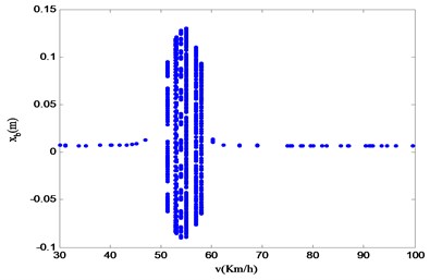
It is assumed that the vehicle enters the continuous SCHs at a speed of 30.00 km/h, and the speed will change within the 30.00 km/h-100.00 km/h interval after entering. the speed bifurcation diagram of the system is drawn and analyzed to study its nonlinear dynamic characteristics, and obtain the speed range of its periodic motion and complex motion. Fig. 17 shows the velocity bifurcation diagram of the 4-DOF variables.

This section assumes that the vehicle enters the consecutive SCHs at a speed of 30.00 km/h, and then the speed will change within the speed range of 30.00 km/h-100.00 km/h. In order to analyze the chaotic vibration of the system, it was required to draw and analyze the velocity bifurcation diagram of the system through calculation. As a result the velocity interval of periodic motion and complex motion of the system is obtained [13]. The velocity bifurcation diagram is shown in Fig. 17.

By analyzing the velocity bifurcation diagram in Fig. 17, the authors of this paper find that different system state variables will reflect similar nonlinear dynamic characteristics within a certain velocity range. The speed modes are divided into the following three regions based on the difference of nonlinear motion characteristics: A (30.00 km/h-46.94 km/h), B (51.32 km/h-57.97 km/h), and C (57.97 km/h-100.00 km/h). Looking at Fig. 17, it is possible to find that the difference between the velocity bifurcation diagrams of the state variable $θ$ and ones of other variables is the most obvious. Therefore, the parameter $θ$ is taken here as the representative for studying the nonlinear vibration of the vehicle. In order to study the nonlinear vibration characteristics of system within the range of 30.00 km/h $\leq v \leq$ 100.00 km/h, the paper selected speeds of $v =$ 44.27 km/h, $v =$ 53.08 km/h and $v =$ 90.06 km/h in the three regions. In order to better analyze the nonlinear motion characteristics of suspension system, the phase diagram of system state variables $θ$ at different speeds, Poincaré mapping, time history and power spectrum at different speeds are calculated as shown in Fig. 18-20.

Fig. 17Speed bifurcation diagram of 4-DOF variables

a) Velocity bifurcation diagram of vertical displacement $x_{b}$ of vehicle body

b) Velocity bifurcation diagram of pitch angle $θ$ of vehicle body

c) Velocity bifurcation diagram of vertical displacement $x_{f}$ of vehicle’s front wheel

d) Velocity bifurcation diagram of vertical displacement $x_{r}$

It can be seen from Fig. 18 that in region A (30.00 km/h~46.94 km/h), the phase diagram of the state variable $θ$ is composed of multiple closed curves, the Poincaré section shows countless points randomly distributed; the time history shows non-periodic changes; the logarithmic power spectrum is distributed in a continuous form. According to the nonlinear feature extraction method, it can be known that the system state variables $θ$ do chaotic vibration at a speed of $v =$ 44.27 km/h. It can be further concluded that the nonlinear motion mode of the system in region A is chaotic motion.

It can be seen from Fig. 19 that in the region B (51.32 km/h-57.97 km/h), the phase diagram of the state variable $θ$ is composed of a twisted combination of countless similar loops; a closed loop is mapped on the Poincaré section; the time history is stable as a whole; and the logarithmic power spectrum is complex. According to the nonlinear feature extraction method, it can be known that the nonlinear motion of the system state variable $θ$ at a speed of $v =$ 53.08 km/h and is accompanied with quasi-periodic vibration. So it can be further concluded that the nonlinear motion of the system in region B is quasi-periodic motion.

Fig. 18Phase portrait, Poincaré map, time history and power spectrum of θ at v= 44.27 km/h

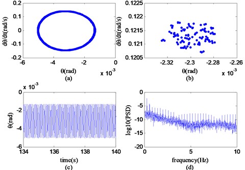
Fig. 19Phase portrait, Poincaré map, time history and power spectrum of θ at v= 53.08 km/h

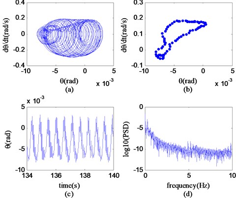
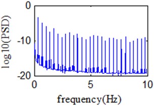
Fig. 20Phase portrait, Poincaré map, time history and power spectrum of θ at v= 91.06 km/h

It can be seen from Fig. 20 that in the region C (57.97 km/h-100.00 km/h), the phase diagram of the state variable $θ$ is composed of countless overlapping closed curves and fills the entire phase space; the Poincaré section has an infinite number of points; the time history shows a non-periodic change; the logarithmic line of the power spectrum is continuously distributed. According to the nonlinear feature extraction method, it can be known that the nonlinear motion mode of the system state variable at a speed of $v =$ 91.06 km/h is chaotic motion. It can be further concluded that the non-linear motion in the region C is chaotic motion.

Through the above analysis, when the vehicle moves on the continuous SCHs with variable acceleration, affected by combined excitation of the consecutive SCHs and uneven road, the nonlinear motion law of the vehicle suspension system is: chaotic motion → quasi periodic motion → chaotic motion. It can be seen that when the vehicle passes through the consecutive SCHs with variable acceleration, the vehicle suspension system has the possibility of chaos. As the vehicle speed increases, the motion state of the vehicle changes from chaotic motion state to chaotic motion.

In Section 5.1, the motion law of vehicle passing consecutive SCHs with variable deceleration is chaotic motion (100.00 km/h-62.25 km/h) → transition state (60.28 km/h-59.49 km/h) → quasi-periodic motion (58.70 km/h-50.79 km/h) → periodic motion (48.68 km/h-30.00 km/h). When the vehicle passes through the consecutive SCHs with variable acceleration, the motion law is chaotic motion A (30.00 km/h-46.94 km/h) → quasi-periodic motion B (51.32 km/h-57.97 km/h) → chaotic motion C (57.97 km/h-100.00 km/h). The critical condition for chaotic vibration of deceleration motion is $v =$ 100.00 km/h. The critical conditions for chaotic vibration of accelerated motion are $v =$ 30.00 km/h and $v =$ 57.97 km/h. The same range of chaotic motion in the two cases is (100.00 km/h-62.25 km/h). By comparing the nonlinear dynamic characteristics of acceleration and deceleration through continuous SCH, it is possible to come to the following conclusions:

1) Whether it is accelerating or decelerating, chaotic motion may occur, and its critical conditions are similar.

2) There will be periodic movement when the vehicle decelerates and passes through a SCH, and then it does not exist when it accelerates. As a conclusion, it is not suitable for the driver to speed up when passing a continuous SCH.

6. Conclusions

This paper mainly compares and analyzes the nonlinear dynamic characteristics of a vehicle passing continuous SCHs at a constant speed with acceleration and deceleration, establishes a nonlinear 4-DOF vehicle suspension model and the continuous SCHs speed coupling excitation model, and adopts the means for numerical simulation and the nonlinear feature extraction method. It can be seen from the results that in the three cases, chaotic motion is possible to occur when the vehicle passes through the continuous SCHs. Among them, the critical speed of chaotic vibration when the vehicle accelerates to 100 km/h, and the critical speed when decelerates to 30 km/h and 57.97 km/h. Based on a comparative analysis, the following conclusions were made:

1) When the vehicle moves on the uneven road at a uniform speed, the chaotic motion will be caused by the rupture of the quasi periodic ring, and its nonlinear motion law is: periodic motion → quasi-periodic motion → chaotic motion.

2) When the vehicle decelerates when moving on the uneven road, its law is: chaotic motion →transition state →quasi-periodic motion → periodic motion.

3) When the vehicle accelerates when moving on the uneven road, the law is: chaotic motion → quasi-periodic motion → chaotic motion.

4) Chaotic motion may occur when the vehicle both at a constant speed and variable speed moves on uneven roads, and there are similar critical speeds.

5) Periodic movement will occur when decelerating through uneven road surface, but not when accelerating, so it is inappropriate to accelerate on the uneven road surface.

This conclusion will provide theoretical support for the adaptive speed regulation through the expressway continuous SCHs in the automatic driving scene. In the follow-up, the authors will further study how to reduce or avoid chaotic motion, and explore the optimal speed range when passing the SCHs, so as to improve passenger safety and comfort.

References

H. Zhang, E. Wang, F. Min, and N. Zhang, “Hysteresis-induced bifurcation and chaos in a magneto-rheological suspension system under external excitation,” Chinese Physics B, Vol. 25, No. 3, pp. 030503–30503, Mar. 2016, https://doi.org/10.1088/1674-1056/25/3/030503

Publisher
L. Zhao, J. Guo, Y. Yu, X. Li, and C. Zhou, “Simulation of nonlinear vibration responses of cab system subject to suspension damper complete failure for trucks,” International Journal of Modeling, Simulation, and Scientific Computing, Vol. 11, No. 2, p. 2050017, Apr. 2020, https://doi.org/10.1142/s1793962320500178

Publisher
A. Sezgin and Y. Z. Arslan, “Analysis of vertical vibration effects on ride comfort of vehicle driver,” Journal of Vibroengineering, Vol. 14, No. 2, pp. 559–571, 2012.

Search CrossRef
J. Fakhraei, H. M. Khanlo, and R. Dehghani, “Nonlinear dynamic behavior of a heavy articulated vehicle with magnetorheological dampers,” Journal of Computational and Nonlinear Dynamics, Vol. 12, No. 4, Jul. 2017, https://doi.org/10.1115/1.4035669

Publisher
G. Litak, M. Borowiec, M. I. Friswell, and W. Przystupa, “Chaotic response of a quarter car model forced by a road profile with a stochastic component,” Chaos, Solitons and Fractals, Vol. 39, No. 5, pp. 2448–2456, 2009.

Publisher
H. Liu, K. Nonami, and T. Hagiwara, “Semi-active fuzzy sliding mode control of full vehicle and suspensions,” Journal of Vibration and Control, Vol. 11, No. 8, pp. 1025–1042, Aug. 2005, https://doi.org/10.1177/1077546305053399

Publisher
Q. Zhu and M. Ishitobi, “Chaotic vibration of a nonlinear full-vehicle model,” International Journal of Solids and Structures, Vol. 43, No. 3-4, pp. 747–759, Feb. 2006, https://doi.org/10.1016/j.ijsolstr.2005.06.070

Publisher
Z. Yang, S. Liang, Q. Zhu, Y. Sun, and S. Zhan, “Chaotic vibration and comfort analysis of nonlinear half-vehicle mode excited by consecutive speed-control humps,” Journal of Robotics and Mechatronics, Vol. 27, No. 5, pp. 513–519, Oct. 2015, https://doi.org/10.20965/jrm.2015.p0513

Publisher
Q. Zhu and M. Ishitobi, “Chaotic oscillations of a nonlinear two degrees of freedom system with air springs,” Dynamics of Continuous Discrete and Impulsive Systems: Series B, Vol. 14, No. 1, pp. 123–133, 2007.

Search CrossRef
Z. Yang, S. Liang, Y. Sun, and Q. Zhu, “Vibration suppression of four degree-of-freedom nonlinear vehicle suspension model excited by the consecutive speed humps,” Journal of Vibration and Control, Vol. 22, No. 6, pp. 1560–1567, Apr. 2016, https://doi.org/10.1177/1077546314543728

Publisher
W. Wang, M. Niu, and Y. Song, “Integrated vibration control of in-wheel motor-suspensions coupling system via dynamics parameter optimization,” Shock and Vibration, Vol. 2019, pp. 1–14, Aug. 2019, https://doi.org/10.1155/2019/3702919

Publisher
Zhiyong Yang, S. Liang, Yongsheng Sun, and Qin Zhu, “Chaotic vibration and control in nonlinear half-vehicle suspension under consecutive humps excitation,” in 2014 International Conference on Advanced Mechatronic Systems, 2014.

Publisher
Y. Zhou and Z. Yang, “The nonlinear dynamic analysis of vehicle variable-speed passing consecutive speed control humps,” in 2018 International Conference on Advanced Mechatronic Systems (ICAMechS), pp. 227–232, Aug. 2018, https://doi.org/10.1109/icamechs.2018.8506787

Publisher

Cited by

Investigation of Driving Stability of a Vehicle–Trailer Combination Depending on the Load’s Position Within the Trailer

(2023)

Research on adaptive speed control method of an autonomous vehicle passing a speed bump on the highway based on a genetic algorithm

Long Wang | Zhiyong Yang | Xiangdong Chen | Ruixiang Zhang | Yu Zhou

(2022)

About this article

Received

13 October 2021

Accepted

26 February 2022

Published

30 June 2022

SUBJECTS

Vibration in transportation engineering

DOI

https://doi.org/10.21595/jve.2022.22250

Keywords

autonomous vehicle

nonlinear dynamic

consecutive SCHs

constant-speed

variable-speed

4-DOF

Acknowledgements

The author is very grateful to the anonymous reviewer for his/her useful comments and suggestions, and the Fundamental Research Funds for the Program for Innovation Research Groups at Institutions of Higher Education in Chongqing (CXQT21032), and the Fundamental Research Funds for the Science and Technology Research Project of Chongqing Municipal Education Commission, China (KJQN201903402), and the Fundamental Research Funds for the Natural Science Foundation of Chongqing, China (cstc2021ycjh-bgzxm0088) for support.

This is an open access article distributed under the Creative Commons Attribution License, which permits unrestricted use, distribution, and reproduction in any medium, provided the original work is properly cited.

Previous article in issue Previous Next article in issue Next

Research article

2023 08 01

Minimum-time lane changing problem of vehicle handling inverse dynamics based on adaptive mesh refinement and collocation optimization method

Yingjie Liu, Dawei Cui, Wen Peng

Research article

2022 12 11

Vehicle state and parameter estimation based on adaptive robust unscented particle filter

Yingjie Liu, Dawei Cui, Wen Peng

Research article

2019 09 30

Collaborative model analysis on ride comfort and handling stability

Yingjie Liu, Dawei Cui

Research article

2017 03 31

Levitation chassis dynamic analysis and robust position control for maglev vehicles under nonlinear periodic disturbance

Haiyan Qiang, Wanli Li, Yougang Sun, Xiangyong Liu

Z. Yang, L. Wang, F. Liu, and Z. Li, “Nonlinear dynamic analysis of constant-speed and variable-speed of autonomous vehicle passing uneven road,” Journal of Vibroengineering, Vol. 24, No. 4, pp. 726–744, Jun. 2022, https://doi.org/10.21595/jve.2022.22250

Copy Extrica

Copied to clipboard!

TY  - JOUR
DO  - 10.21595/jve.2022.22250
UR  - https://doi.org/10.21595/jve.2022.22250
TI  - Nonlinear dynamic analysis of constant-speed and variable-speed of autonomous vehicle passing uneven road
T2  - Journal of Vibroengineering
AU  - Yang, Zhiyong
AU  - Wang, Long
AU  - Liu, Fangtao
AU  - Li, Zijian
PY  - 2022
DA  - 2022/06/30
PB  - JVE International Ltd.
SP  - 726-744
VL  - 24
IS  - 4
SN  - 1392-8716
SN  - 2538-8460
ER  - 

Copy Ris

Copied to clipboard!

@article{Yang_2022,
	doi = {10.21595/jve.2022.22250},
	url = {https://doi.org/10.21595/jve.2022.22250},
	year = 2022,
	month = {mar},
	publisher = {{JVE} International Ltd.},
	volume = {24},
	number = {4},
	pages = {726--744},
	author = {Zhiyong Yang and Long Wang and Fangtao Liu and Zijian Li},
	title = {Nonlinear dynamic analysis of constant-speed and variable-speed of autonomous vehicle passing uneven road},
	journal = {Journal of Vibroengineering}
}

Copy Bibtex

Copied to clipboard!

[1]Z. Yang, L. Wang, F. Liu, and Z. Li, “Nonlinear dynamic analysis of constant-speed and variable-speed of autonomous vehicle passing uneven road,” Journal of Vibroengineering, vol. 24, no. 4, pp. 726–744, Mar. 2022, doi: 10.21595/jve.2022.22250.

Copy IEEE

Copied to clipboard!

Yang, Zhiyong, Long Wang, Fangtao Liu, and Zijian Li. “Nonlinear Dynamic Analysis of Constant-Speed and Variable-Speed of Autonomous Vehicle Passing Uneven Road.” Journal of Vibroengineering 24, no. 4 (March 16, 2022): 726–44. https://doi.org/10.21595/jve.2022.22250.

Copy Chicago

Copied to clipboard!

Nonlinear dynamic analysis of constant-speed and variable-speed of autonomous vehicle passing uneven road

Abstract

Highlights

1. Introduction

2. Simulation model description

2.1. Nonlinear 4-DOF half-vehicle model

2.2. Excitation model of consecutive SCHs

2.3. Instantaneous speed representation

2.4. Simulation parameters

3. Nonlinear feature extraction method

3.1. Bifurcation diagram

3.2. Phase portrait

3.3. Poincaré map

3.4. Time history

3.5. Power spectrum

4. Analysis of nonlinear dynamic characteristics of vehicles moving on uneven road surface at constant speed

5. Analysis of nonlinear dynamic characteristics of vehicles moving on uneven road at variable speed

5.1. Analysis of nonlinear dynamic characteristics during vehicle deceleration through consecutive SCHs

5.2. Analysis of nonlinear dynamic characteristics of vehicle acceleration through consecutive SCHs

6. Conclusions

References

Cited by

About this article

Related Articles