Active vibration suppression of a nonlinear electromechanical oscillator system with simultaneous resonance

Hamed, Y. S.; Sayed, M.; Alshehri, A. A.

doi:10.21595/jve.2017.18261

Journal of Vibroengineering

Browse Journal

Submit article

Published: 15 February 2018

Check for updates

Active vibration suppression of a nonlinear electromechanical oscillator system with simultaneous resonance

Y. S. Hamed¹

M. Sayed²

A. A. Alshehri³

^{1, 2}Department of Physics and Engineering Mathematics, Faculty of Electronic Engineering, Menoufia University, Menouf, 32952, Egypt

^{1, 2}Department of Mathematics and Statistics, Faculty of Science, Taif University, Taif, El-Haweiah, P.O. Box 888, 21974, Kingdom of Saudi Arabia

³Department of Mathematics, Faculty of Sciences and Arts in ALnamas, Bisha University, P.O. Box 555, 61922, Kingdom of Saudi Arabia

Corresponding Author:

Y. S. Hamed

Cite the article Download PDF

Downloads 1669

WoS Core Citations 6

CrossRef Citations 6

Abstract

In this paper, we explored the nonlinear dynamics behavior and vibration suppression of a nonlinear electromechanical oscillator system under harmonic and parametric excitation. The model comprises of an electrical part coupled to mechanical part and displayed by a coupled nonlinear ordinary differential equations. The analytical up to second order approximate solutions are sought applying the method of multiple scales method. We utilized the time-series and method of averaging to analyze the response and stability of the solutions at the worst resonance cases. We checked the results of perturbation solution through numerical simulations and the effects of different system parameters have been reported. Comparison between analytical and numerical solutions is obtained. Also, the numerical results are obtained using MAPLE and MATLAB algorisms.

1. Introduction

Controlling nonlinear coupling between vibrating modes are critical for the development of advanced nano-mechanical or micro-electromechanical devices. The coupled oscillators give principal models for the dynamics of different physical, biological, chemical and engineering systems. The nonlinear electromechanical oscillator systems consist of an electrical part as a sign component of the measured vibration coupled magnetically to a mechanical part as a sensor communicate through the air-gap of a permanent magnet. Yamapi et al. [1] studied the stability, oscillations and chaos control in a nonlinear electromechanical system. Ge and Lin [2] studied dynamic behavior, synchronization and chaos control (delayed feedback control, adaptive control) of electromechanical gyrostat system subjected to external disturbance. Yamapi and Bowong [3] examined the dynamic behavior and chaos control of a self-sustained electromechanical system without and with discontinuity and they utilized a sliding mode controller to control the electrostatic transducers system. Siewe et al. [4] used an electromechanical oscillator system to record the vertical movement of earth during earthquake. Also, they examined the chaos control of the system using small amplitude damping. They found that the chaotic and periodic orbits depend on the estimation of the damping coefficient. Yamapi et al. [5, 6] investigated the dynamics and synchronization of two systems, one of them is a coupled self-sustained electromechanical systems with multiple functions and the other is an electrical Rayleigh–Duffing oscillator coupled magnetically with linear mechanical oscillators. They established the amplitudes of the oscillatory states applying the harmonic balance and averaging methods. Kwuimy and Woafo [7, 8] studied the chaotic behavior, global bifurcations and dynamics of a self-sustained of non-linear electromechanical systems with nonlinear. Ngueuteu et al. [9] investigated the effects of higher nonlinearity parameters on the synchronization and dynamics of coupled electromechanical system. Hegazy [10] investigated the chaotic motions and nonlinear vibrations in an electromechanical seismograph system with time-varying stiffness. He used different types of active controllers to reduce the system oscillations and he found that the negative velocity feedback is the best active control on the system behavior. Siewe et al. [11] used an analytical method based on the Melnikov theory to investigate the bifurcation and control of homoclinic orbits in electromechanical seismographs with cubic-nonlinearities. Kwuimy and Woafo [12] presented simulations and an experimental investigation of a self-sustained electromechanical system. The considered system was made up of an electrical execution of a van der Pol-Duffing oscillator through a macro scale mass–spring–damper linear oscillator. Siewe and Buckjohn [13] investigated the heteroclinic motion associated to a Melnikov-like investigation, energy transfer, and harvesting in coupled oscillator with nonlinear magnetic coupling. Amer [14] studied the behavior, stability, approximate solutions, active feedback control of a nonlinear electromechanical seismograph system with time-varying stiffness and he compared the numerical solution with perturbation one. Eissa et al. [15] investigated the effects of saturation phenomena on nonlinear oscillating systems under multi-parametric or external excitation forces. Also, the occurrence of saturation phenomena at different parameters values was studied. Eissa et al. [16-18] used a negative velocity feedback or square or cubic feedback to control the vibration of simple and spring pendulum system at the primary resonance. Amer et al. [19] investigated and control the behavior of a twin-tail aircraft system having both quadratic and cubic nonlinearities. Hamed et al. [20-22] used a passive vibration control on the ultrasonic machining system with multi types of excitation forces. Kamel and Hamed [23] utilized the multiple scale technique to investigate the vibrations behavior of the inclined cable system with harmonic excitation at the simultaneous of primary and internal resonance cases. Hamed et al. [24] investigated the behavior of vibrations for the nonlinear string beam system under external, parametric and tuned excitations forces. Sayed and Hamed [25] presented a mathematical study for the analytical, numerical solutions and stability of a coupled pitch roll system to harmonic and parametric excitation forces. Sayed and Kamel [26, 27] used the saturation control of a linear controller to reduce the vibrations due to rotor blade flapping motion and they investigated the effect of different controllers on the vibrating system. Sayed et al. [28-31] investigated the non-linear dynamic characteristics of the angle-ply composite laminated rectangular plate model under both parametric and external excitations. Also, they studied three cases of primary and internal resonance (1:2, 1:1, 1:1:3) and they compared the analytical results with the numerical one of the modal equations. Hamed and Amer [32] used different types of control algorithms and studied its effectiveness to reduce the large vibrations of a flexible composite beam system. Hamed et al. [33] studied the stability and nonlinear oscillations of the MEMS gyroscope system under different types of parametric excitations. The averaging method has been used to obtain the frequency response equations at simultaneous resonance case. We can find a detailed analysis of dynamical systems excited by external and parametric forces in the books of Cartmell [34], Nayfeh and Balachandran [35]. In the present paper, the nonlinear dynamics and vibration suppression of a nonlinear electromechanical system under harmonic and parametric excitations are investigated. The time-series and method of averaging [36] to analyze the response and stability of the solutions at the worst resonance cases were utilized. the results of perturbation solution through numerical simulations and the effects of different system parameters have been reported. Comparison between analytical and numerical solutions is obtained.

2. Description of the system with equations of motion

Fig. 1 showed the scheme of the investigated electromechanical oscillator system. The electromechanical device modeling consist of two parts electrical and mechanical. the electrical part consists of a linear inductor $L$ , a linear capacitor $C$ , a linear resistor $R$ , and voltage-charge $q$ . The mechanical part is composed of a large suspended mass. The mechanical and electrical parts interact through the air-gap of a permanent magnet which creates a radial magnetic field $B$ which given in the appendix.

The nonlinear differential equations corresponding to the system in Fig. 1 may be obtained using Newton’s second law and Kirchhoff’s law. Thus, the complete mathematical model [13] that describes the dynamics of the system is governed by the following nonlinear differential equations:

1

\{\begin{array}{l} m \ddot{y} + μ_{0} \dot{y} + k_{0} y + k_{1} y^{3} = F_{c} + F (t), \\ L \ddot{q} + R \dot{q} + \frac{1}{C} q + E_{b e m f} = 0, \end{array}

where $y$ is the relative displacement of the mass $m$ with inertial forces $m \ddot{y}$ and damping forces $μ_{0} \dot{y}$ and $k_{0}$ , $k_{1}$ are linear and nonlinear stiffness of the electromechanical oscillator system; $k_{1} < 0,$ the external ground motion is assumed to be stochastic or periodic $(F (t) = F_{0} + F_{1} c o s (Ω_{1} t) + F_{2} y c o s (Ω_{2} t))$ where $F_{0}$ is the critical amplitude, $F_{1} c o s (Ω_{1} t)$ is the external force, with amplitude $F_{1}$ and $Ω_{1}$ the excitation frequency, $F_{2} y c o s (Ω_{2} t)$ is the parametric force, with amplitude $F_{2}$ and $Ω_{2}$ the excitation frequency. We address the case where the critical value of the force is zero, and this means $F_{0} =$ 0 in the corresponding equation.

We put system Eq. (1) into dimensionless form by setting: $x = y / l$ , $z = q / Q_{0}$ where $Q_{0}$ is the reference charge and $l$ is the reference length. By introducing the characteristic parameters of the system:

ω_{e}^{2} = \frac{1}{L C}, ω_{m}^{2} = \frac{k_{0}}{m}, μ_{1} = \frac{μ_{0}}{m ω_{e}}, μ_{2} = \frac{R}{L ω_{e}} .

And using the time transformation $τ = ω_{e} t$ .

In the mechanical part $F_{c}$ is the relationship between the force and the current and $E_{b e m f}$ is the Lenz electromotive voltage in the electrical part and they are defined in the appendix.

The mathematical model [13] described the dynamics of the electromechanical oscillator system and the following dimensionless form of system Eq. (1) is obtained and governed by the following nonlinear differential equations:

2a

\ddot{x} + ε μ_{1} \dot{x} + ω_{1}^{2} x - ε α_{1} x^{3} + ε (γ_{1} + γ_{2} x + γ_{3} x^{2}) \dot{z} = ε f_{1} c o s (Ω_{1} τ) + ε f_{2} x c o s (Ω_{2} τ),

2b

\ddot{z} + ε μ_{2} \dot{z} + ω_{2}^{2} z + ε (β_{1} + β_{2} x + β_{3} x^{2}) \dot{x} = 0 .

With initial conditions $x (0) = 0.01$ , $\dot{x} (0) = 0$ , $z (0) = 0$ , $\dot{z} (0) = 0$ ., and the parameters of Eqs. (2a) and (2b) are defined as:

ω_{1} = \frac{ω_{m}}{ω_{e}}, α_{1} = \frac{|k_{1}|}{m l^{2} ω_{e}^{2}},

f_{1} = \frac{F_{1}}{m l ω_{e}^{2}}, f_{2} = \frac{F_{2}}{m l ω_{e}^{2}}, γ_{1} = \frac{α_{0}}{m l ω_{e}^{2}} (\frac{y_{0}^{2}}{y_{m a x}^{2}} - 1), γ_{2} = \frac{2 y_{0} α_{0}}{m ω_{e}^{2} y_{m a x}},

γ_{3} = \frac{l α_{0}}{m ω_{e}^{2} y_{m a x}^{2}}, β_{1} = \frac{- k_{0}}{L l ω_{e}^{2}} (\frac{y_{0}^{2}}{y_{m a x}^{2}} - 1), β_{2} = \frac{- 2 y_{0} α_{0}}{L ω_{e}^{2} y_{m a x}}, β_{3} = \frac{- l α_{0}}{L ω_{e}^{2} y_{m a x}^{2}} .

The first oscillator $x$ (mechanical part) is a forced Duffing oscillator associated with nonlinear coupling term, and the second one $z$ (electrical part) is a linear damped oscillator with nonlinear coupling term. $\dot{x}$ , $\dot{z}$ , $\ddot{x}$ and $\ddot{z}$ are the first and second derivative with respect to time $t$ , $μ_{1}$ and $μ_{2}$ are linear damping coefficients, $α_{1}$ is non-linear parameters, $ε$ is a small perturbation where $0 < ε ≪ 1$ , $f_{1}$ , $f_{2}$ are the amplitudes of excitation force $ω_{1}$ , $ω_{2}$ are the natural frequencies and $Ω_{1}$ , $Ω_{2}$ are excitation frequencies, $γ_{j}$ and $β_{j}$ ( $j =$ 1, 2, 3)are the coupling terms.

Fig. 1Schematic of electromechanical model with the associated electric circuit [13]

3. Mathematical analysis

In this section, we applied the multiple scale perturbation and averaging method [35, 37] to obtain the approximate solutions and frequency response equations respectively.

3.1. Perturbation analysis

To obtain the approximate solutions for Eq. (2a) and (2b), we used the multiple scale perturbation method. Assuming the solution to be in the form:

3

\{\begin{array}{l} x (t; ε) = x_{0} (T_{0}, T_{1}) + ε x_{1} (T_{0}, T_{1}) + O (ε^{2}), \\ z (t; ε) = z_{0} (T_{0}, T_{1}) + ε z_{1} (T_{0}, T_{1}) + O (ε^{2}) . \end{array}

We introduced the derivatives in the form:

4

\{\begin{array}{l} \frac{d}{d t} = D_{0} + ε D_{1} + \dots, \\ \frac{d^{2}}{d t^{2}} = D_{0}^{2} + 2 ε D_{0} D_{1} + \dots . \end{array}

For the approximate solutions, we introduce two time scales, where $T_{n} = ε^{n} t$ and the derivatives $D_{n} = \partial / \partial T_{n}$ , ( $n =$ 0, 1). Substituting Eqs. (3), (4) into Eqs. (2a) and (2b) and equating the coefficients of powers of $ε$ leads to:

5

(D_{0}^{2} + ω_{1}^{2}) x_{0} = 0,

6

({D_{0}}^{2} + ω_{2}^{2}) z_{0} = 0,

7

({D_{0}}^{2} + {ω_{1}}^{2}) x_{1} = - 2 D_{0} D_{1} x_{0} - μ_{1} D_{0} x_{0} + α_{1} x_{0}^{3} - γ_{1} D_{0} z_{0} - γ_{2} x_{0} D_{0} z_{0} - γ_{3} x_{0}^{2} D_{0} z_{0}

+ f_{1} c o s (Ω_{1} t) + f_{2} x_{0} c o s (Ω_{2} t),

8

(D_{0}^{2} + ω_{2}^{2}) z_{1} = - 2 D_{0} D_{1} z_{0} - μ_{2} D_{0} z_{0} - β_{1} D_{0} x_{0} - β_{2} x_{0} D_{0} x_{0} - β_{3} x_{0}^{2} D_{0} x_{0} .

The differential Eqs. (5) and (6) have the general solutions:

9

x_{0} = A_{0} e x p (i ω_{1} T_{0}) + {\bar{A}}_{0} e x p (- i ω_{1} T_{0}),

10

z_{0} = B_{0} e x p (i ω_{2} T_{0}) + {\bar{B}}_{0} e x p (- i ω_{2} T_{0}),

where $A_{0}$ , ${\bar{A}}_{0}$ , $B_{0}$ and ${\bar{B}}_{0}$ are complex functions in $T_{1}$ . Substituting Eq. (9) and (10) into Eq. (7) and (8), and eliminated the coefficients of the secular terms, thus the general solutions will be in the form:

11

x_{1} = A_{1} e x p (i ω_{1} T_{0}) + {\bar{A}}_{1} e x p (- i ω_{1} T_{0}) - \frac{α_{1}}{8 ω_{1}^{2}} (A_{0}^{3} e x p (3 i ω_{1} T_{0}) + {\bar{A}}_{0}^{3} e x p (- 3 i ω_{1} T_{0}))

+ \frac{1}{ω_{1}^{2} - ω_{2}^{2}} (- γ_{1} i ω_{2} B_{0} - 2 γ_{3} i ω_{2} A_{0} {\bar{A}}_{0} B_{0}) e x p (i ω_{2} T_{0})

+ \frac{1}{ω_{1}^{2} - ω_{2}^{2}} (γ_{1} i ω_{2} {\bar{B}}_{0} + 2 γ_{3} i ω_{2} A_{0} {\bar{A}}_{0} {\bar{B}}_{0}) e x p (- i ω_{2} T_{0})

+ \frac{1}{ω_{1}^{2} - {(ω_{1} + ω_{2})}^{2}} [\begin{matrix} - γ_{2} i ω_{2} A_{0} B_{0} e x p (i T_{0} (ω_{1} + ω_{2})) \\ + γ_{2} i ω_{2} {\bar{A}}_{0} {\bar{B}}_{0} e x p (- i T_{0} (ω_{1} + ω_{2})) \end{matrix}]

+ \frac{1}{ω_{1}^{2} - {(ω_{1} - ω_{2})}^{2}} [\begin{matrix} γ_{2} i ω_{2} A_{0} {\bar{B}}_{0} e x p (i T_{0} (ω_{1} - ω_{2})) \\ - γ_{2} i ω_{2} {\bar{A}}_{0} B_{0} e x p (- i T_{0} (ω_{1} - ω_{2})) \end{matrix}]

+ \frac{1}{ω_{1}^{2} - {(2 ω_{1} + ω_{2})}^{2}} [\begin{matrix} - γ_{3} i ω_{2} {A_{0}}^{2} B_{0} e x p (i T_{0} (2 ω_{1} + ω_{2})) \\ + γ_{3} i ω_{2} {\bar{A}}_{0}^{2} {\bar{B}}_{0} e x p (- i T_{0} (2 ω_{1} - ω_{2})) \end{matrix}]

+ \frac{1}{ω_{1}^{2} - {(2 ω_{1} - ω_{2})}^{2}} [\begin{matrix} γ_{3} i ω_{2} {A_{0}}^{2} {\bar{B}}_{0} e x p (i T_{0} (2 ω_{1} - ω_{2})) \\ - γ_{3} i ω_{2} {\bar{A}}_{0}^{2} B_{0} e x p (- i T_{0} (2 ω_{1} - ω_{2})) \end{matrix}]

+ \frac{f_{1}}{2 (ω_{1}^{2} - Ω_{1}^{2})} e x p (i Ω_{1} T) +_{0} \frac{f_{1}}{2 (ω_{1}^{2} + Ω_{1}^{2})} e x p (- i Ω_{2} T_{0})

+ \frac{f_{2}}{2 (ω_{1}^{2} - {(Ω_{2} + ω_{1})}^{2})} A_{0} e x p (i T_{0} (Ω_{2} + ω_{1}))

+ \frac{f_{2}}{2 (ω_{1}^{2} - {(Ω_{2} + ω_{1})}^{2})} {\bar{A}}_{0} e x p (- i T_{0} (Ω_{2} + ω_{1}))

+ \frac{f_{2}}{2 (ω_{1}^{2} - {(Ω_{2} - ω_{1})}^{2})} {\bar{A}}_{0} e x p (i T_{0} (Ω_{2} - ω_{1}))

+ \frac{f_{2}}{2 (ω_{1}^{2} - {(Ω_{2} - ω_{1})}^{2})} A_{0} e x p (- i T_{0} (Ω_{2} - ω_{1})),

12

z_{1} = B_{1} e x p (i ω_{2} T_{0}) + {\bar{B}}_{1} e x p (- i ω_{2} T_{0})

+ \frac{1}{ω_{2}^{2} - ω_{1}^{2}} (\begin{matrix} - β_{1} i ω_{1} A_{0} - β_{3} i ω_{1} {A_{0}}^{2} {\bar{A}}_{0} \end{matrix}) e x p (i ω_{1} T_{0})

+ \frac{1}{ω_{2}^{2} - ω_{1}^{2}} (β_{1} i ω_{1} {\bar{A}}_{0} + β_{3} i ω_{1} A_{0} {\bar{A}}_{0}^{2}) e x p (- i ω_{1} T_{0})

+ \frac{1}{ω_{2}^{2} - 4 ω_{1}^{2}} (- β_{2} i ω_{1} A_{0}^{2} e x p (2 i ω_{1} T_{0}) + β_{2} i ω_{1} {\bar{A}}_{0}^{2} e x p (- 2 i ω_{1} T_{0}))

+ \frac{1}{ω_{2}^{2} - 9 ω_{1}^{2}} (- β_{2} i ω_{1} {A_{0}}^{3} e x p (3 i ω_{1} T_{0}) + β_{2} i ω_{1} {\bar{A}}_{0}^{3} e x p (- 3 i ω_{1} T_{0})),

where $A_{1}$ , ${\bar{A}}_{1}$ , $B_{1}$ and ${\bar{B}}_{1}$ are complex functions in $T_{1}$ .

From the derived approximate solutions, we extracted all resonance cases and reported it as the following:

a) Primary resonance: $Ω_{1} = \pm ω_{s}$ , $Ω_{2} = \pm ω_{s}$ ; ( $s =$ 1, 2),

b) Sub-harmonic resonance: $Ω_{2} = \pm n ω_{1}$ ; $(n =$ 2, 4 $)$ , $Ω_{1} = \pm 3 ω_{1}$ ,

c) Internal resonance: $ω_{1} = \pm n ω_{2}$ ; ( $n =$ 1, 2), $ω_{2} = \pm m ω_{1}$ ; ( $m =$ 1, 2, 3, 4, 5), $2 ω_{2} = \pm 3 ω_{1}$ ,

d) Combined resonance: $Ω_{1} = \pm (n ω_{1} \pm ω_{2})$ ; ( $n =$ 1, 2), $Ω_{2} = \pm (m ω_{1} \pm ω_{2})$ ; ( $m =$ 1, 2, 3), $\pm ω_{1} \pm ω_{2} = \pm ω_{1}$ .

3.2. Averaging method

The averaging method is applied to obtain the frequency response equations for Eqs. (2a) and (2b). When $ε =$ 0, the general solution of Eqs. (2a) and (2b) can be expressed as:

13

x = a_{1} c o s (ω_{1} t + φ_{1}),

14

z = a_{2} c o s (ω_{2} t + φ_{2}),

where $a_{1}$ , $a_{2}$ , $φ_{1}$ and $φ_{2}$ are constants. It follows from Eqs. (13), (14) that:

15

\dot{x} = - ω_{1} a_{1} s i n (ω_{1} t + φ_{1}),

16

\dot{z} = - ω_{2} a_{2} s i n (ω_{2} t + φ_{2}) .

For $ε \neq$ 0 small enough, let $a_{1}$ , $a_{2}$ , $φ_{1}$ and $φ_{2}$ are unknown function of time $t$ in Eqs. (2a) and (2b).

We derivative the Eqs. (13) and (14) with respect to $t$ yields:

17

\dot{x} = {\dot{a}}_{1} c o s (ω_{1} t + φ_{1}) - ω_{1} a_{1} s i n (ω_{1} t + φ_{1}) - a_{1} {\dot{φ}}_{1} s i n (ω_{1} t + φ_{1}),

18

\dot{z} = {\dot{a}}_{2} c o s (ω_{2} t + φ_{2}) - ω_{2} a_{2} s i n (ω_{2} t + φ_{2}) - a_{2} {\dot{φ}}_{2} s i n (ω_{2} t + φ_{2}) .

Comparing Eqs. (15), (16) and (17), (18), we conclude that:

19

{\dot{a}}_{1} c o s (ω_{1} t + φ_{1}) - a_{1} {\dot{φ}}_{1} s i n (ω_{1} t + φ_{1}) = 0,

20

{\dot{a}}_{2} c o s (ω_{2} t + φ_{2}) - a_{2} {\dot{φ}}_{2} s i n (ω_{2} t + φ_{2}) = 0 .

Differentiating Eqs. (15) and (16) with respect to $t$ , we have:

21

\ddot{x} = - ω_{1} {\dot{a}}_{1} s i n (ω_{1} t + φ_{1}) - ω_{1}^{2} a_{1} c o s (ω_{1} t + φ_{1}) - ω_{1} a_{1} {\dot{φ}}_{1} c o s (ω_{1} t + φ_{1}),

22

\ddot{z} = - ω_{2} {\dot{a}}_{2} s i n (ω_{2} t + φ_{2}) - ω_{2}^{2} a_{2} c o s (ω_{2} t + φ_{2}) - ω_{2} a_{2} {\dot{φ}}_{2} c o s (ω_{2} t + φ_{2}) .

Inserting for $x$ , $z$ , $\dot{x}$ , $\dot{z}$ , $\ddot{x}$ and $\ddot{z}$ from Eqs. (13)-(22) into Eqs. (2a) and (2b), we obtain:

23

{\dot{a}}_{1} s i n (ω_{1} t + φ_{1}) + a_{1} {\dot{φ}}_{1} c o s (ω_{1} t + φ_{1}) + ε μ_{1} a_{1} s i n (ω_{1} t + φ_{1}) + \frac{ε α_{1} a_{1}^{3}}{ω_{1}} c o s^{3} (ω_{1} t + φ_{1})

+ \frac{ε γ_{1} a_{2} ω_{2}}{ω_{1}} s i n (ω_{2} t + φ_{2}) + \frac{ε γ_{2} a_{1} a_{2} ω_{2}}{ω_{1}} c o s (ω_{1} t + φ_{1}) s i n (ω_{2} t + φ_{2})

+ \frac{ε γ_{3} a_{1}^{2} a_{2} ω_{2}}{ω_{1}} c o s^{2} (ω_{1} t + φ_{1}) s i n (ω_{2} t + φ_{2}) = \frac{- ε f_{1}}{ω_{1}} c o s (Ω_{1} t)

- \frac{ε f_{2} a_{1}}{ω_{1}} c o s (ω_{1} t + φ_{1}) c o s (Ω_{2} t),

24

{\dot{a}}_{2} s i n (ω_{2} t + φ_{2}) + a_{2} {\dot{φ}}_{2} c o s (ω_{2} t + φ_{2}) + ε μ_{2} a_{2} s i n (ω_{2} t + φ_{2})

+ \frac{ε β_{1} a_{1} ω_{1}}{ω_{2}} s i n (ω_{1} t + φ_{1}) + \frac{ε β_{2} a_{1}^{2} ω_{1}}{ω_{2}} c o s (ω_{1} t + φ_{1}) s i n (ω_{1} t + φ_{1})

+ \frac{ε β_{3} a_{2}^{3} ω_{1}}{ω_{2}} c o s^{2} (ω_{1} t + φ_{1}) s i n (ω_{1} t + φ_{1}) = 0 .

Substituting Eqs. (19), (20) into Eqs. (23), (24) and solving it for $a_{1}$ , $a_{2}$ , $φ_{1}$ and $φ_{2}$ yield:

25

{\dot{a}}_{1} = \frac{- ε μ_{1} a_{1}}{2} (1 - c o s (2 ω_{1} t + 2 φ_{1}))

- \frac{ε α_{1} a_{1}^{3}}{ω_{1}} \frac{1}{8} (\begin{matrix} s i n (4 ω_{1} t + 4 φ_{1}) + \frac{1}{4} s i n (2 ω_{1} t + 2 φ_{1}) \end{matrix})

+ \frac{ε γ_{1} ω_{2} a_{2}}{2 ω_{1}} [c o s ((ω_{2} + ω_{1}) t + φ_{2} + φ_{1}) - c o s ((ω_{1} - ω_{2}) t + φ_{1} - φ_{2})]

+ \frac{ε γ_{2} ω_{2} a_{1} a_{2}}{4 ω_{1}} [c o s ((ω_{2} + 2 ω_{1}) t + φ_{2} + 2 φ_{1}) - c o s (2 ω_{1} - ω_{2}) t + 2 φ_{1} - φ_{2}]

+ \frac{ε γ_{3} ω_{2} a_{1}^{2} a_{2}}{8 ω_{1}} [c o s ((ω_{1} + ω_{2}) t + φ_{1} + φ_{2}) - c o s ((3 ω_{1} - ω_{2}) t + 3 φ_{1} - φ_{2})]

- [c o s ((ω_{1} - ω_{2}) t + φ_{1} - φ_{2}) + c o s ((3 ω_{1} + ω_{2}) t + 3 φ_{1} + φ_{2})]

- \frac{ε f_{1}}{2 ω_{1}} [s i n ((Ω_{1} + ω_{1}) t + φ_{1}) - s i n ((Ω_{1} - ω_{1}) t - φ_{1})]

- \frac{ε f_{2} a_{1}}{4 ω_{1}} [s i n ((Ω_{2} + 2 ω_{1}) t + 2 φ_{1}) - s i n ((Ω_{2} - 2 ω_{1}) t - 2 φ_{1})],

26

a_{1} {\dot{φ}}_{1} = \frac{- ε μ_{1} a_{1}}{2} (s i n (2 ω_{1} t + 2 φ_{1}))

- \frac{ε α_{1} a_{1}^{3}}{ω_{1}} (\begin{matrix} \frac{3}{8} + \frac{1}{8} c o s (4 ω_{1} t + 4 φ_{1}) + \frac{1}{2} c o s (2 ω_{1} t + 2 φ_{1}) \end{matrix})

- \frac{ε γ_{1} ω_{2} a_{2}}{2 ω_{1}} [s i n ((ω_{2} + ω_{1}) t + φ_{2} + φ_{1}) - s i n ((ω_{1} - ω_{2}) t + φ_{1} - φ_{2})]

- \frac{ε γ_{2} ω_{2} a_{1} a_{2}}{2 ω_{1}} [s i n (ω_{2} t + φ_{2}) + \frac{1}{2} s i n (\begin{matrix} (ω_{2} + 2 ω_{1}) t \\ + φ_{2} + 2 φ_{1} \end{matrix}) - \frac{1}{2} s i n (\begin{matrix} (2 ω_{1} - ω_{2}) t \\ + 2 φ_{1} - φ_{2} \end{matrix})]

- \frac{ε γ_{3} ω_{2} a_{1}^{2} a_{2}}{8 ω_{1}} [s i n ((3 ω_{1} + ω_{2}) t + 3 φ_{1} + φ_{2}) - s i n ((3 ω_{1} - ω_{2}) t + 3 φ_{1} - φ_{2})

+ 3 s i n ((ω_{1} + ω_{2}) t + φ_{1} + φ_{2}) - 3 s i n ((ω_{1} - ω_{2}) t + φ_{1} - φ_{2})]

- \frac{ε f_{1}}{2 ω_{1}} [c o s ((Ω_{1} + ω_{1}) t + φ_{1}) + c o s ((Ω_{1} - ω_{1}) t - φ_{1})]

- \frac{ε f_{2} a_{1}}{2 ω_{1}} [c o s (Ω_{2} t) + \frac{1}{2} c o s ((Ω_{2} + 2 ω_{1}) t + 2 φ_{1}) + \frac{1}{2} c o s ((Ω_{2} - 2 ω_{1}) t - 2 φ_{1})],

27

{\dot{a}}_{2} = \frac{- ε μ_{2} a_{2}}{2} (1 - (c o s 2 ω_{2} t + 2 φ_{2}))

+ \frac{ε β_{1} ω_{1} a_{1}}{2 ω_{2}} [\begin{matrix} c o s ((ω_{2} + ω_{1}) t + φ_{2} + φ_{1}) - c o s ((ω_{1} - ω_{2}) t + φ_{1} - φ_{2}) \end{matrix}]

+ \frac{ε β_{2} ω_{1} a_{1}^{2}}{4 ω_{2}} (c o s ((ω_{2} + 2 ω_{1}) t + φ_{2} + 2 φ_{1}) - c o s ((2 ω_{1} - ω_{2}) t + 2 φ_{1} - φ_{2}))

+ \frac{ε β_{3} ω_{1} a_{2}^{3}}{8 ω_{2}} [c o s ((ω_{1} + ω_{2}) t + φ_{1} + φ_{2}) - c o s ((3 ω_{1} - ω_{2}) t + 3 φ_{1} - φ_{2})

- c o s ((ω_{1} - ω_{2}) t + φ_{1} - φ_{2}) + c o s ((3 ω_{1} + ω_{2}) t + 3 φ_{1} + φ_{2})],

28

a_{2} {\dot{φ}}_{2} = \frac{- ε μ_{2} a_{2}}{2} (s i n (2 ω_{2} t + 2 φ_{2}))

- \frac{ε β_{1} ω_{2} a_{1}}{2 ω_{2}} [\begin{matrix} s i n ((ω_{2} + ω_{1}) t + φ_{2} + φ_{1}) + s i n ((ω_{1} - ω_{2}) t + φ_{1} - φ_{2}) \end{matrix}]

- \frac{ε β_{2} ω_{1} a_{1}^{2}}{4 ω_{2}} [s i n ((2 ω_{1} - ω_{2}) t + 2 φ_{1} - φ_{2}) + s i n ((2 ω_{1} + ω_{2}) t + 2 φ_{1} + φ_{2})]

- \frac{ε β_{3} ω_{1} a_{2}^{3}}{8 ω_{2}} [s i n ((2 ω_{1} - ω_{2}) t + 2 φ_{1} - φ_{2}) + s i n ((ω_{1} - ω_{2}) t + φ_{1} - φ_{2})

+ s i n ((3 ω_{1} - ω_{2}) t + 3 φ_{1} - φ_{2}) + s i n ((ω_{1} + ω_{2}) t + φ_{1} + φ_{2})] .

3.3. Periodic solutions

In this section, we obtained the averaging equations corresponding to simultaneous primary, sub-harmonic and internal resonance by utilizing the detuning parameters ( $σ_{1}$ , $σ_{2}$ , $σ_{3}$ ) as:

Ω_{1} = ω_{1} + ε σ_{1}, Ω_{2} = 2 ω_{1} + ε σ_{2}, ω_{2} = ω_{1} + ε σ_{3} .

And keeping only the constant terms and slowly varying parts in Eqs. (25)-(28), we have:

29

{\dot{a}}_{1}^{} = - \frac{μ_{1}}{2} a_{1} - \frac{γ_{1} ω_{2}}{2 ω_{1}} a_{2} c o s θ_{3} - \frac{γ_{3} ω_{2}}{4 ω_{1}} a_{1}^{2} a_{2} c o s θ_{3}

+ \frac{γ_{3} ω_{2}}{8 ω_{1}} a_{1}^{2} a_{2} c o s θ_{3} + \frac{f_{1}}{2 ω_{1}} s i n θ_{1} + \frac{f_{2}}{4 ω_{1}} a_{1} s i n θ_{2},

30

{\dot{φ}}_{1} a_{1} = - \frac{3 α_{1}}{8 ω_{1}} a_{1}^{3} - \frac{γ_{1} ω_{2}}{2 ω_{1}} a_{2} s i n θ_{3} - \frac{γ_{3} ω_{2}}{4 ω_{1}} a_{1}^{2} a_{2} s i n θ_{3}

- \frac{γ_{3} ω_{2}}{8 ω_{1}} a_{1}^{2} a_{2} s i n θ_{3} - \frac{f_{1}}{2 ω_{1}} c o s θ_{1} - \frac{f_{2}}{4 ω_{1}} a_{1} c o s θ_{2},

31

{\dot{a}}_{2} = - \frac{μ_{2}}{2} a_{2} - \frac{β_{1} ω_{1}}{2 ω_{2}} a_{1} c o s θ_{3} - \frac{β_{3} ω_{1}}{8 ω_{2}} a_{1}^{3} c o s θ_{3},

32

{\dot{φ}}_{2} a_{2} = \frac{β_{1} ω_{1}}{2 ω_{2}} a_{1} s i n θ_{3} + \frac{β_{3} ω_{1}}{8 ω_{2}} a_{1}^{3} s i n θ_{3},

where:

θ_{1} = σ_{1} T_{1} - φ_{1}, θ_{2} = σ_{2} T_{1} - 2 φ_{1}, θ_{3} = φ_{2} - φ_{1} + σ_{3} T_{1} .

We can have written the first approximation periodic solution in the form:

33

x = a_{1} c o s (Ω_{1} t - θ_{1}),

34

z = a_{2} c o s (Ω_{1} t + θ_{3}),

where $a_{1}$ , $a_{2}$ , $θ_{1}$ , $θ_{2}$ and $θ_{3}$ are the solutions of Eqs. (29)-(32).

3.4. Stability of the fixed points

We obtained the fixed point of the dynamical system of Eqs. (29)-(32) when ${\dot{a}}_{m} =$ 0, ( $m =$ 1, 2) and ${\dot{θ}}_{n} =$ 0, where ( $n =$ 1, 3) as the following:

35

\frac{μ_{1}}{2} a_{1} = - \frac{γ_{1} ω_{2}}{2 ω_{1}} a_{2} c o s θ_{3} - \frac{γ_{3} ω_{2}}{4 ω_{1}} a_{1}^{2} a_{2} c o s θ_{3}

+ \frac{γ_{3} ω_{2}}{8 ω_{1}} a_{1}^{2} a_{2} c o s θ_{3} + \frac{f_{1}}{2 ω_{1}} s i n θ_{1} + \frac{f_{2}}{4 ω_{1}} a_{1} s i n θ_{2},

36

a_{1} σ + \frac{3 α_{1}}{8 ω_{1}} a_{1}^{3} = - \frac{γ_{1} ω_{2}}{2 ω_{1}} a_{2} s i n θ_{3} - \frac{γ_{3} ω_{2}}{4 ω_{1}} a_{1}^{2} a_{2} s i n θ_{3}

- \frac{γ_{3} ω_{2}}{8 ω_{1}} a_{1}^{2} a_{2} s i n θ_{3} - \frac{f_{1}}{2 ω_{1}} c o s θ_{1} - \frac{f_{2}}{4 ω_{1}} a_{1} c o s θ_{2},

37

\frac{μ_{2}}{2} a_{2} = - \frac{β_{1} ω_{1}}{2 ω_{2}} a_{1} c o s θ_{3} - \frac{β_{3} ω_{1}}{8 ω_{2}} a_{1}^{3} c o s θ_{3},

38

a_{2} (σ - σ_{3}) = \frac{β_{1} ω_{1}}{2 ω_{2}} a_{1} s i n θ_{3} + \frac{β_{3} ω_{1}}{8 ω_{2}} a_{1}^{3} s i n θ_{3} .

Where $σ = σ_{1} = σ_{2} / 2$ . For the case ( $a_{1} \neq$ 0, $a_{2} \neq$ 0), the frequency response equations are given by:

39

(a_{1}^{2} + \frac{9 γ_{3}^{2} ω_{2}^{4} a_{1}^{2} a_{2}^{4}}{ω_{1}^{4} {(4 β_{1} + a_{1}^{2} β_{3})}^{2}} + \frac{24 γ_{1} ω_{2}^{4} a_{2}^{4} γ_{2}}{ω_{1}^{4} {(4 β_{1} + a_{1}^{2} β_{3})}^{2}} + \frac{8 γ_{1} ω_{2}^{2} a_{2}^{2}}{ω_{1}^{2} (4 β_{1} + a_{1}^{2} β_{3})} + \frac{16 γ_{1}^{2} ω_{2}^{4} a_{2}^{2}}{a_{1}^{2} ω_{1}^{4} {(4 β_{1} + a_{1}^{2} β_{3})}^{2}}

+ \frac{6 a_{1}^{2} a_{2}^{2} γ_{3} ω_{2}^{2}}{ω_{1}^{2} (4 β_{1} + a_{1}^{2} β_{3})}) σ^{2} - (\frac{48 γ_{1} ω_{2}^{4} a_{2}^{4} γ_{2} σ_{3}}{ω_{1}^{4} {(4 β_{1} + a_{1}^{2} β_{3})}^{2}} - \frac{8 γ_{1} ω_{2}^{2} a_{2}^{2} σ_{3}}{ω_{1}^{2} (4 β_{1} + a_{1}^{2} β_{3})} - \frac{18 γ_{3}^{2} ω_{2}^{4} a_{1}^{2} a_{2}^{4} σ_{3}}{ω_{1}^{4} {(4 β_{1} + a_{1}^{2} β_{3})}^{2}}

+ \frac{3 α_{1} a_{1}^{2} γ_{1} ω_{2}^{2} a_{2}^{2}}{ω_{1}^{3} (4 β_{1} + a_{1}^{2} β_{3})} + \frac{9 α_{1} a_{1}^{4} γ_{3} ω_{2}^{2} a_{2}^{2}}{4 ω_{1}^{3} (4 β_{1} + a_{1}^{2} β_{3})} - \frac{32 γ_{1}^{2} ω_{2}^{4} a_{2}^{4} σ_{3}}{a_{1}^{2} ω_{1}^{4} {(4 β_{1} + a_{1}^{2} β_{3})}^{2}} - \frac{6 a_{1}^{2} γ_{3} ω_{2}^{2} a_{2}^{2} σ_{3}}{ω_{1}^{2} (4 β_{1} + a_{1}^{2} β_{3})}

+ \frac{3 α_{1} a_{1}^{4}}{4 ω_{1}}) σ + (\frac{16 γ_{1}^{2} ω_{2}^{4} a_{2}^{4} σ_{3}^{2}}{a_{1}^{2} ω_{1}^{4} {(4 β_{1} + a_{1}^{2} β_{3})}^{2}} + \frac{24 γ_{1} ω_{2}^{4} a_{2}^{4} σ_{3}^{2} γ_{2}}{ω_{1}^{4} {(4 β_{1} + a_{1}^{2} β_{3})}^{2}} - \frac{1}{4} \frac{f_{1}^{2}}{ω_{1}^{2}} + \frac{9 α_{1}^{2} a_{1}^{6}}{64 ω_{1}^{2}} - \frac{1}{16} \frac{f_{2}^{2} a_{1}^{2}}{ω_{1}^{2}}

+ \frac{2 γ_{1} ω_{2}^{4} a_{2}^{4} μ_{2}^{2} γ_{3}}{ω_{1}^{4} {(4 β_{1} + a_{1}^{2} β_{3})}^{2}} - \frac{2 μ_{1} γ_{1} ω_{2}^{2} a_{2}^{2} μ_{2}}{ω_{1}^{2} (4 β_{1} + a_{1}^{2} β_{3})} - \frac{1}{2} \frac{μ_{1} a_{1}^{2} γ_{3} ω_{2}^{2} a_{2}^{2} μ_{2}}{ω_{1}^{2} (4 β_{1} + a_{1}^{2} β_{3})} + \frac{4 γ_{1}^{2} ω_{2}^{4} a_{2}^{4} μ_{2}^{2}}{a_{1}^{2} ω_{1}^{4} {(4 β_{1} + a_{1}^{2} β_{3})}^{2}}

+ \frac{1}{4} \frac{γ_{3}^{2} a_{1}^{2} ω_{2}^{4} a_{2}^{4} μ_{2}^{2}}{ω_{1}^{4} {(4 β_{1} + a_{1}^{2} β_{3})}^{2}} - \frac{3 α_{1} a_{1}^{2} γ_{1} ω_{2}^{2} a_{2}^{2} σ_{3}}{ω_{1}^{3} (4 β_{1} + a_{1}^{2} β_{3})} - \frac{9}{4} \frac{α_{1} a_{1}^{4} γ_{3} ω_{2}^{2} a_{2}^{2} σ_{3}}{ω_{1}^{3} (4 β_{1} + a_{1}^{2} β_{3})} + \frac{9 γ_{3}^{2} ω_{2}^{4} a_{1}^{2} a_{2}^{4} σ_{3}^{2}}{ω_{1}^{4} {(4 β_{1} + a_{1}^{2} β_{3})}^{2}}

+ \frac{1}{4} μ_{1}^{2} a_{1}^{2} - \frac{1}{4} \frac{f_{1} f_{2} a_{1}}{ω_{1}^{2}}) = 0,

40

a_{2}^{2} σ_{3}^{2} + (- 2 σ a_{2}^{2}) σ_{3} + (σ^{2} a_{2}^{2} + \frac{μ_{2}^{2}}{4} a_{2}^{2} - a_{2}^{2} \frac{β_{1}^{2} ω_{1}^{2}}{4 ω_{2}^{2}} a_{1}^{2} - \frac{β_{3}^{2} ω_{1}^{2}}{64 ω_{2}^{2}} a_{2}^{2} a_{1}^{6} - \frac{β_{1} β_{3} ω_{1}^{2}}{8 ω_{2}^{2}} a_{2}^{2} a_{1}^{4}) = 0 .

To study the stability of the nonlinear solution, we lets:

41

a_{m} = a_{m 0} + a_{m 1}, θ_{n} = θ_{n 0} + θ_{n 1},

where $a_{m 0}$ and $θ_{n 0}$ are the solutions of Eq. (29)-(32), ( $m =$ 1, 2) and ( $n =$ 1, 3). Inserting Eq. (41) into Eqs. (29)-(32) and linearizing equations in $a_{m 1}$ and $θ_{n 1}$ , we get:

42

{\dot{a}}_{11} = [- \frac{μ_{1}}{2} - \frac{γ_{3} ω_{2}}{2 ω_{1}} a_{10} a_{20} c o s θ_{20} + \frac{γ_{3} ω_{2}}{4 ω_{1}} a_{10} a_{20} c o s θ_{20} + \frac{f_{2}}{2 ω_{1}} s i n 2 θ_{10}] a_{11} + [\frac{f_{1}}{2 ω_{1}} c o s θ_{10} + \frac{f_{2}}{2 ω_{1}} a_{10} c o s 2 θ_{10}] θ_{11} + [\frac{γ_{1} ω_{2}}{2 ω_{1}} a_{20} s i n θ_{30} + \frac{γ_{3} ω_{2}}{4 ω_{1}} a_{10}^{2} a_{20} s i n θ_{30} - \frac{γ_{3} ω_{2}}{8 ω_{1}} a_{10}^{2} a_{20} s i n θ_{30}] θ_{31},

43

{\dot{θ}}_{11} = [\frac{σ}{a_{10}} + \frac{9 α_{1}}{8 ω_{1}} a_{10} + \frac{γ_{3} ω_{2}}{2 ω_{1}} a_{20} s i n θ_{30} + \frac{γ_{3} ω_{2}}{4 ω_{1}} a_{20} s i n θ_{30} + \frac{f_{2}}{4 ω_{1} a_{10}} c o s 2 θ_{10}] a_{11}

+ [\frac{- f_{1}}{2 ω_{1} a_{10}} s i n θ_{10} - \frac{f_{2}}{2 ω_{1}} s i n 2 θ_{10}] θ_{11}

+ [\begin{matrix} \frac{γ_{1} ω_{2}}{2 ω_{1} a_{10}} s i n θ_{30} + \frac{γ_{3} ω_{2}}{4 ω_{1}} a_{10} s i n θ_{30} + \frac{γ_{3} ω_{2}}{8 ω_{1}} a_{10} s i n θ_{30} \end{matrix}] a_{21} + [\frac{γ_{1} ω_{2}}{2 ω_{1} a_{10}} a_{20} c o s θ_{30} + \frac{γ_{3} ω_{2}}{4 ω_{1}} a_{10} a_{20} c o s θ_{30} + \frac{γ_{3} ω_{2}}{8 ω_{1}} a_{10} a_{20} s i n θ_{30}] θ_{31},

44

{\dot{a}}_{21} = [\frac{- β_{1} ω_{1}}{2 ω_{2}} c o s θ_{30} - \frac{3 β_{3} ω_{1}}{8 ω_{2}} a_{10}^{2} c o s θ_{30}] a_{11} - \frac{μ_{2}}{2} a_{21} + [\frac{β_{1} ω_{1}}{2 ω_{2}} a_{10} s i n θ_{30} + \frac{β_{3} ω_{1}}{8 ω_{2}} a_{10}^{3} s i n θ_{30}] θ_{31},

45

{\dot{θ}}_{31} = [\frac{σ_{3}}{a_{10}} + \frac{9 α_{1}}{8 ω_{1}} a_{10} + \frac{3 γ_{3} ω_{2}}{4 ω_{1}} a_{20} s i n θ_{30} + \frac{f_{2}}{4 ω_{1} a_{10}} c o s 2 θ_{10}

+ \frac{β_{1} ω_{1}}{ω_{2} a_{20}} s i n θ_{30} + \frac{β_{3} ω_{1}}{2 ω_{2} a_{20}} a_{10}^{2} s i n θ_{30}] a_{11} + [\frac{- f_{1}}{2 ω_{1} a_{10}} s i n θ_{10} - \frac{f_{2}}{2 ω_{1}} s i n 2 θ_{10}] θ_{11} + [\frac{σ_{3}}{a_{20}} + \frac{9 α_{1}}{8 ω_{1}} a_{10} + \frac{γ_{1} ω_{2}}{ω_{1} a_{10}} s i n θ_{30} + \frac{γ_{3} ω_{2}}{4 ω_{1}} a_{10} s i n θ_{30} + \frac{3 γ_{3} ω_{2}}{4 ω_{1}} a_{10} s i n θ_{30} + \frac{f_{1}}{2 ω_{1} a_{10} a_{20}} c o s θ_{10} + \frac{f_{2}}{4 ω_{1} a_{20}} c o s 2 θ_{10}] a_{21} + [\frac{γ_{1} ω_{2}}{2 ω_{1} a_{10}} a_{20} c o s θ_{30} + \frac{3 γ_{3} ω_{2}}{8 ω_{1}} a_{10} a_{20} c o s θ_{30} + \frac{ω_{1} β_{3}}{8 ω_{2} a_{20}} a_{10}^{3} c o s θ_{30} + \frac{ω_{1} β_{1}}{2 ω_{2} a_{20}} a_{10} c o s θ_{30}] θ_{31} .

The system of Eqs. (42)-(45) has an eigenvalues and are given by the equation:

46

λ^{4} + r_{1} λ^{3} + r_{2} λ^{2} + r_{3} λ + r_{4} = 0,

where $r_{1}$ , $r_{2}$ , $r_{3}$ and $r_{4}$ are constants and given in the Appendix. The periodic solution of the system is stable, if the real part of the eigenvalue is negative; otherwise become unstable. As indicated by the Routh-Huriwitz criterion, the necessary and sufficient conditions for all the roots of Eq. (46) to have negative real parts (asymptotically stable system), are if and only if the following equation is satisfied:

47

r_{1} > 0, r_{1} r_{2} - r_{3} > 0, r_{3} (r_{1} r_{2} - r_{3}) - r_{1}^{2} r_{4} > 0, r_{4} > 0 .

4. Results and discussion

Within this section, the results are presented in graphical forms as steady state amplitudes ( $a_{1}$ , $a_{2}$ ) against detuning parameters ( $σ_{1}$ , $σ_{2}$ ) and the time response for both an electromechanical system and controller. The system original Eqs. (2a) and (2b) have been solved numerically using ODE45 MATLAB solver. The numerical solution of the mathematical modeling and its stability is studied here and the solutions of the frequency response function regarding the stability of the electromechanical system and the controller are examined. The effects of various parameters on the steady state solution are obtained and studied also different resonance cases are reported and discussed.

4.1. System behavior and frequency response curves

In this section, the figures demonstrating the effects of different electromechanical oscillator system and controller parameters on the whole system behavior are gotten. All the derived resonance cases from Eqs. (11) and (12) are studied numerically. The analysis is performed by adopting the following values of the system parameters:

μ_{1} = 0.06, μ_{2} = 0.006, α_{1} = 0.002, ε = 1, ω_{1} = 3, Ω_{1} = ω_{1}, Ω_{2} = 2 ω_{1},

f_{1} = 0.2, f_{2} = 0.02, γ_{1} = 0.2, γ_{2} = 0.25, γ_{3} = 0.5,

β_{1} = - 0.2, β_{2} = - 0.25, β_{3} = - 0.5 .

We summarized the results of worst cases in Table 1. From this table, the worst results have been obtained for the simultaneous primary, sub-harmonic and internal resonance case $Ω_{1} = ω_{1}$ , $Ω_{2} = 2 ω_{1}$ and $ω_{2} = ω_{1}$ .

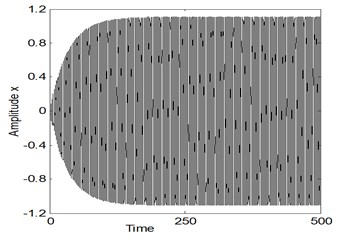
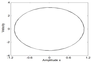
Fig. 2. represents the system time histories and the phase-plane for the electromechanical system before control at the simultaneous primary and sub-harmonic resonance case where $Ω_{1} = ω_{1}$ , $Ω_{2} = 2 ω_{1}$ . It is noticed from this figure that the steady state amplitude of the main system is about 560 % of the greatest excitation force amplitude $f_{1}$ , the oscillation response begins with increasing amplitude and becomes stable and the phase plane shows limit cycle.

For the uncontrolled system, where $a_{1} \neq$ 0, $a_{2} =$ 0. Fig. 3(a) shows the steady state amplitude of the electromechanical system against the detuning parameters $σ_{1}$ , the system responds as a linear system. It is clear that the greatest steady state amplitude occurs at simultaneous primary and sub-harmonic resonance case $Ω_{1} = ω_{1}$ , $Ω_{2} = 2 ω_{1}$ (where $σ_{1} =$ 0). Figs. 3(b) and 3(c) illustrates that the steady state amplitude of the system is inversely proportional to the linear damping coefficients $μ_{1}$ and the natural frequency $ω_{1}$ . Fig. 3(d) shows the effects of the non-linear parameters $α_{1}$ , we note that from Fig. 3(d), for the negative and positive values of $α_{1}$ , the curve is either bent to the right or to the left leading to the existence of the jump phenomenon and producing either hard or soft spring respectively. Fig. 3(e) and 3(f) shows that the steady state amplitude a₁ is directly proportional to the external and parametric excitation forces $f_{1}$ and $f_{2}$ . Also, for increasing excitation forces the curve is bent to the left and we obtain unstable region.

Fig. 2The response amplitude of the electromechanical system before control at the case Ω 1=ω1, Ω 2=2ω1

a)

b)

Table 1Summaries of the worst resonance cases of the electromechanical system and controller

Case	Condition	Amplitude ration ( $x / f_{1}$ ) without controller	Amplitude ration ( $x / f_{1}$ ) with controller	Amplitude ration ( $z / f_{1}$ )	$E_{a}$
$Ω_{1} = ω_{1}$ $Ω_{2} = ω_{1}$	$ω_{1} = ω_{2}$	550 %	8 %	160 %	70
	$ω_{1} = {2 ω}_{2}$	550 %	400 %	50 %	38
	$ω_{2} = {2 ω}_{1}$	550 %	400 %	225 %	38
	$ω_{2} = {3 ω}_{1}$	550 %	350 %	75 %	58
	$ω_{2} = {4 ω}_{1}$	550 %	550 %	9 %	1
	$ω_{2} = {5 ω}_{1}$	550 %	550 %	5 %	1
	3 $ω_{1} = {2 ω}_{2}$	550 %	450 %	45 %	22
$Ω_{1} = ω_{1}$ $Ω_{2} = {2 ω}_{1}$	$ω_{1} = ω_{2}$	560 %	5 %	165 %	110
	$ω_{1} = {2 ω}_{2}$	560 %	400 %	50 %	4
	$ω_{2} = {2 ω}_{1}$	560 %	400 %	225 %	4
	$ω_{2} = {3 ω}_{1}$	560 %	350 %	75 %	6
	$ω_{2} = {4 ω}_{1}$	560 %	550 %	8.5 %	1
	$ω_{2} = {5 ω}_{1}$	560 %	550 %	4.5 %	1
	3 $ω_{1} = {2 ω}_{2}$	560 %	450 %	45 %	25
$Ω_{1} = ω_{1}$ $Ω_{2} = {4 ω}_{1}$	$ω_{1} = ω_{2}$	555 %	5 %	165 %	110
	$ω_{1} = {2 ω}_{2}$	555 %	400 %	225 %	4
	$ω_{2} = {2 ω}_{1}$	555 %	350 %	75 %	6
	$ω_{2} = {3 ω}_{1}$	555 %	550 %	8.5 %	1
	$ω_{2} = {4 ω}_{1}$	555 %	550 %	4.5 %	1
	$ω_{2} = {5 ω}_{1}$	555 %	450 %	45 %	25
	3 $ω_{1} = {2 ω}_{2}$	555 %	400 %	225 %	4

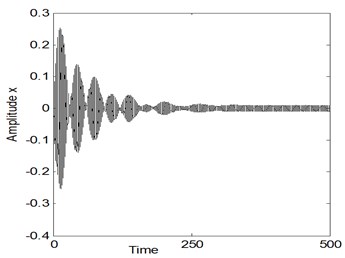
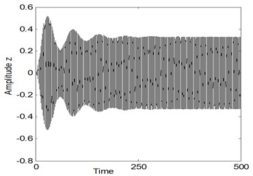
Fig. 4 simulates the system time histories for the electromechanical system after adding the control at simultaneous primary, internal and sub-harmonic resonance case, where $Ω_{1} = ω_{1}$ , $Ω_{2} = 2 ω_{1},$ $ω_{1} = ω_{2} .$ According to this figure, the steady state amplitude for the electromechanical system is 5 %, but the steady state amplitude of the controller is about 165 % of maximum excitation amplitude $f_{1}$ . In addition, the effectiveness of the controller $E_{a}$ ( $E_{a} =$ the steady state amplitude for system before control/the steady state amplitude for the system after control) is about 110.

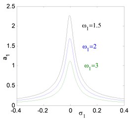
Fig. 5(a), illustrate the steady state amplitudes of the electromechanical system and controller versus the detuning parameter $σ_{1}$ when the controller is in action, where $a_{1} \neq$ 0, $a_{2} \neq$ 0 at similar estimations of parameters appeared in Fig. 4. According to this figure, the minimum steady state amplitude of the main system appear when $σ_{1} =$ 0, which confirms that the controller is able to reduce the vibration effectively and efficiently. Also, Fig. 5(a) indicate that the system has multiple coexisting solutions, and jump phenomenon that occurs in the case of the system became unstable when the controller associated with the system. Fig. 5(b), (c), (d) illustrate that, the steady state amplitude are directly commensurate to external and parametric excitation forces $f_{1}$ , $f_{2}$ and inversely commensurate to the natural frequency $ω_{1}$ .

Fig. 3The frequency-response curves of uncontrolled system

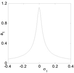
a) Effects of detuning parameters $σ_{1}$

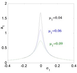
b) Effects of damping coefficient $μ_{1}$

c) Effects of natural frequency $ω_{1}$

d) Effects of the non-linear parameter $α_{1}$

e) Effects of external excitation $f_{1}$

f) Effects of parametric excitation $f_{2}$

Fig. 4The response amplitude of the electromechanical system after control at the case Ω1=ω1, Ω2=2ω1, ω1=ω2, μ1= 0.06, μ2= 0.006, α1= 0.002, ω1= 3, Ω1=ω1, Ω2=2ω1, f1=0.2, f2= 0.02, γ1= 0.2, γ2= 0.25, γ3= 0.5, β1= –0.2, β2= –0.25, β3= –0.5

The response amplitude of the electromechanical system after control at the case Ω1=ω1, Ω2=2ω1, ω1=ω2, μ1= 0.06, μ2= 0.006, α1= 0.002, ω1= 3, Ω1=ω1, Ω2=2ω1, f1=0.2, f2= 0.02, γ1= 0.2, γ2= 0.25, γ3= 0.5, β1= –0.2, β2= –0.25, β3= –0.5

a)

b)

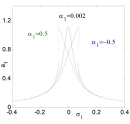
In addition, the regions of instability system are increased for increasing $f_{1}$ , $f_{2}$ and decreasing $ω_{1}$ . Fig. 5(e) and (f), shows the effects of the damping coefficients $μ_{1}$ and $μ_{2}$ on both the electromechanical system and controller. According to this figure, the small values of damping coefficients $μ_{1}$ , $μ_{2}$ the presence of various solution, bifurcation points and jumping phenomenon occurs. In addition, for large values of damping coefficients, both the system and the controller displays linear responses and the jumping phenomenon disappears. It is clear that, as $μ_{1}$ increases, the controller’s efficiency to eliminate the primary, principle parametric resonance excitations slightly decreases, but the electromechanical system and the controller peak amplitudes decreases. For negative value of the nonlinear parameters $α_{1}$ , $β_{1}$ , $β_{3}$ the curve is bent to the right leading to the occurrence of the jump phenomena and multi-valued amplitudes produce hardening spring type as shown in Figs. 5(g), (k) and (l). It is clear that, from Figs. 5(h) and (i) that the steady state amplitude of the system is inversely commensurate to the control gains $γ_{1}$ , $γ_{3}$ .

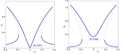
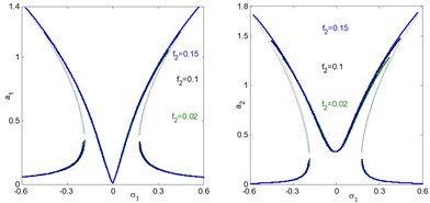
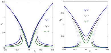
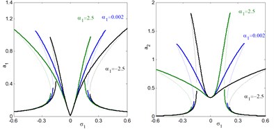
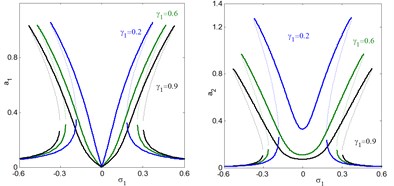
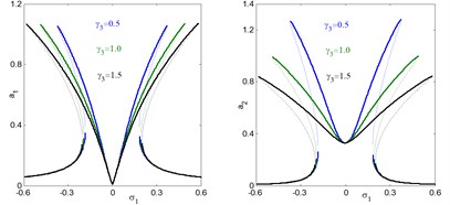
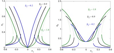
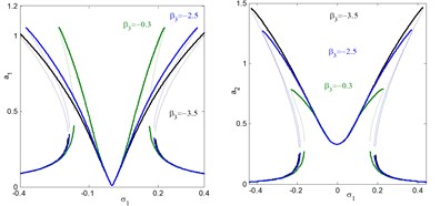
Figs. 6 simulate the frequency response curves of the system after control versus detuning parameter $σ_{3}$ at simultaneous primary, sub-harmonic and internal resonance case $Ω_{1} = ω_{1}$ , $Ω_{2} = 2 ω_{1}$ , $ω_{1} = ω_{2}$ with the same parameters values as shown in Fig. 4. From Figs. 6, we observe that the electromechanical system and controller has continuous curve with stable solution. According to fig. 6(a), we observe that the controller reaches maximum value at $σ_{3} ≅ 0$ and the main system has minimum value at the same value of $σ_{3} ≅$ 0. The electromechanical system and controller intersect with each other in two points.

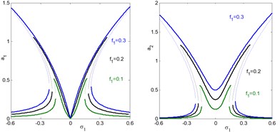
It is clear that from Fig. 6(a) we find that at $σ_{3} ≅$ 0 the amplitudes $a_{1} ≅$ 0.01 and $a_{2} ≅$ 0.33 $.$ These values are very closed to the steady state amplitude of obtained Figs. 4 and 5(a) for $a_{1}$ and $a_{2}$ . For increasing value of external excitation force $f_{1}$ , parametric excitation force $f_{2}$ the electromechanical system and controller have increasing amplitudes, as illustrated in Figs. 6(b) and 6(c). It is clear from Fig. 6(d) that the steady state amplitudes of the main system and controller are decreasing for increasing value of natural frequency.

Fig. 5The frequency-response curves of controlled system (a1 main system, a2 controller) against detuning parameter σ1

a) Effects of detuning parameter $σ_{1}$ on the frequency-response curves of controlled system ( $a_{1}$ main system, $a_{2}$ controller).

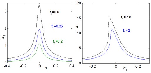
b) Effects of external excitation $f_{1}$ on the controlled system

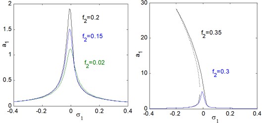
c) Effects of parametric excitation $f_{2}$ on the controlled system

d) Effects of natural frequency $ω_{1}$ on the controlled system

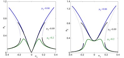
e) Effects of damping coefficient $μ_{1}$ on the controlled system

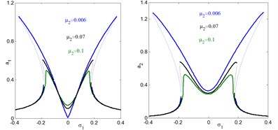
f) Effects of damping coefficient $μ_{2}$ on the controlled system

g) Effects of nonlinear parameter $α_{1}$ on the controlled system

h) Effects of linear control gain $γ_{1}$ on the controlled system

i) Effects of nonlinear control gain $γ_{3}$ on the controlled system

j) Effects of linear control gain $β_{1}$ on the controlled system

k) Effects of nonlinear control gain $β_{3}$ on the controlled system

Fig. 6The frequency response curves of system after control (a1 main system, a2 controller) against detuning parameter σ3

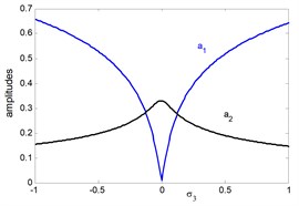
a) Effects of detuning parameter $σ_{3}$ against the frequency response curves of system after control ( $a_{1}$ main system, $a_{2}$ controller)

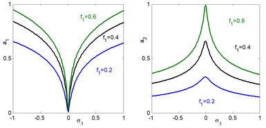
b) Effects of external excitation $f_{1}$ on the controlled system

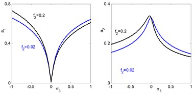
c) Effects of parametric excitation $f_{2}$ on the controlled system

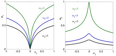
d) Effects of natural frequency $ω_{1}$ on the controlled system

4.2. Comparison study

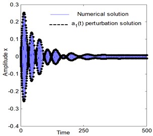
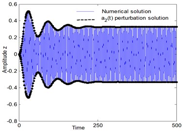
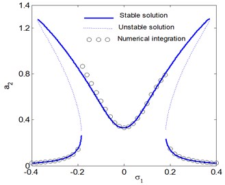
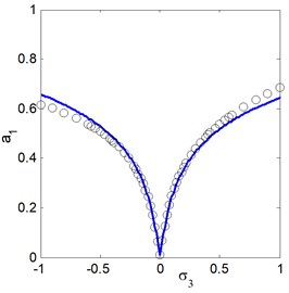
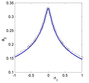
To approve the simulations of perturbation analysis, the analytical results were checked by integration numerically of the Eqs. (2a), (2b), and the numerical outcomes for steady state solutions Fig. 7 indicates a comparison between the time histories and approximate modulated amplitudes of the electromechanical system after control approached by Eqs. (2a), (2b) and (29)-(32) respectively. In addition, Figs. 8, 9 presents a comparison between the frequency response curves for the electromechanical system after control against $σ_{1}$ and $σ_{3}$ respectively with the numerical simulation of Eqs. (2a), (2b) at the same parameters values appear in Fig. 4. Figs. 7-9 illustrate an excellent agreement between the analytical and numerical solutions.

Fig. 7Comparison between numerical simulation (using Runge-Kutta method) and analytical solution (using perturbation method) of the system at resonance case, Ω1≅ω1, Ω2≅2ω1, ω1≅ω2

Comparison between numerical simulation (using Runge-Kutta method) and analytical solution (using perturbation method) of the system at resonance case, Ω1≅ω1, Ω2≅2ω1, ω1≅ω2

a)

b)

4.3. Comparison with published work

In comparison with previous researches, Siewe and Buckjohn [13] investigated the heteroclinic motion, transient chaos and energy transfer from mechanical to electrical oscillators under harmonic excitation. They applied Melnikov method with linear damping and nonlinear coupling terms to study the possibility of existence of chaos and transversal heteroclinic orbits and their control in a dynamical system.

Fig. 8The frequency response curves of the electromechanical system after control at ω1= 4 (a1 main system, a2 controller)

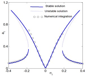
a)

b)

Fig. 9The frequency response curves of the electromechanical system after control (a1 main system, a2 controller)

a)

b)

Within this work, the authors studied the nonlinear dynamics behavior and vibration suppression of a nonlinear electromechanical oscillator system under harmonic and parametric excitation. Also, the authors investigated the energy transfer from mechanical to electrical oscillators Multiple scales perturbations method is applied to obtain the second approximate solutions of this system. The method of averaging is applied to analyze the response and stability of the solutions at the worst resonance cases. In numerical results, the steady state amplitude for the electromechanical system is 5 %, but the steady state amplitude of the controller is about 165 % of maximum excitation amplitude $f_{1}$ and the effectiveness of the controller $E_{a}$ is about 110. Also, jump down phenomenon and multi-valued solutions are appeared using suitable value of system parameters. Finally, the numerical simulations are in good agreement with analytical solutions.

5. Conclusions

An active vibration control is applied to suppress and eliminate the vibrations of a nonlinear electromechanical system under harmonic and parametric excitations. The model comprises of an electrical part coupled to mechanical part and displayed by a coupled nonlinear ordinary differential equations. The analytical up to second order approximate solutions are sought applying the method of multiple scales method. We utilized the time-series and method of averaging to analyze the response and stability of the solutions at the worst resonance cases. We checked the results of perturbation solution through numerical simulations and the effects of different system parameters have been reported. Comparison between analytical and numerical simulations is obtained. According to the above results and discussion, we may conclude the following:

1) In the design of such system, some simultaneous resonance cases should be avoided.

2) For the system before control, the steady state amplitude at simultaneous resonance case $Ω_{1} ≅ ω_{1}$ , $Ω_{2} ≅ 2 ω_{1}$ is about 560 % of the excitation force amplitude $f_{1}$ , which is one of the worst resonance.

3) The effectiveness of the controller $E_{a}$ is about 110.

4) The steady state amplitude is directly commensurate to external and parametric excitation forces $f_{1}$ , $f_{2}$ and inversely commensurate to the natural frequency $ω_{1}$ .

5) For large values of damping coefficients, both the electromechanical system and the controller displays linear responses and the jumping phenomenon disappears.

6) The jump phenomena and multi-valued amplitudes occur and produce hardening spring type for negative value of the nonlinear parameters $α_{1}$ .

7) The steady state amplitude of the system is inversely commensurate to the control gains $γ_{1}$ , $γ_{3}$ .

8) The analytical solutions an excellent agreement with the numerical simulations.

References

Yamapi R., Orou J. B. C., Woafo P. Harmonic oscillations, stability and chaos control in a nonlinear electromechanical system. Journal of Sound and Vibration, Vol. 259, Issue 5, 2003, p. 1253-1264.

Publisher
Ge Z. M., Lin T. N. Chaos, chaos control and synchronization of electro-mechanical gyrostat system. Journal of Sound and Vibration, Vol. 259, Issue 3, 2003, p. 585-603.

Publisher
Yamapi R., Bowong S. Dynamics and chaos control of the self-sustained electromechanical device with and without discontinuity. Communications in Nonlinear Science and Numerical Simulation, Vol. 11, Issue 3, 2006, p. 355-375.

Publisher
Siewe Siewe M., Kakmeni F. M. M., Bowong S., Tchawoua C. Non-linear response of a self-sustained electromechanical seismographs to fifth resonance excitations and chaos control. Chaos Solitons and Fractals, Vol. 29, Issue 2, 2006, p. 431-445.

Publisher
Yamapi R., Kakmeni F. M. M., Orou J. B. C. Nonlinear dynamics and synchronization of coupled electromechanical systems with multiple functions. Communications in Nonlinear Science and Numerical Simulation, Vol. 12, Issue 4, 2007, p. 543-567.

Publisher
Yamapi R., Aziz-Alaoui M. A. Vibration analysis and bifurcations in the self-sustained electromechanical system with multiple functions. Communications in Nonlinear Science and Numerical Simulation, Vol. 12, Issue 8, 2007, p. 1534-1549.

Publisher
Kwuimy C. A. K., Woafo P. Dynamics of a self-sustained electromechanical system with flexible arm and cubic coupling. Communications in Nonlinear Science and Numerical Simulation, Vol. 12, Issue 8, 2007, p. 1504-1517.

Publisher
Kwuimy C. A. K., Woafo P. Dynamics, chaos and synchronization of self-sustained electromechanical systems with clamped-free flexible arm. Nonlinear Dynamics, Vol. 53, Issue 3, 2008, p. 201-213.

Publisher
Ngueuteu G. S. M., Yamapi R., Woafo P. Effects of higher nonlinearity on the dynamics and synchronization of two coupled electromechanical devices. Communications in Nonlinear Science and Numerical Simulation, Vol. 13, Issue 7, 2008, p. 1213-1240.

Publisher
Hegazy U. H. Dynamics and control of a self-sustained electromechanical seismograph with time varying stiffness. Meccanica, Vol. 44, Issue 4, 2009, p. 355-368.

Publisher
Siewe Siewe M., Yamgoué S. B., Moukam Kakmeni F. M., Tchawoua C. Chaos controlling self-sustained electromechanical seismograph system based on the Melnikov theory. Nonlinear Dynnamics, Vol. 62, Issues 1-2, 2010, p. 379-389.

Publisher
Kwuimy C. A. K., Woafo P. Experimental realization and simulations a self-sustained macro electromechanical system. Mechanics Research Communications, Vol. 37, Issue 1, 2010, p. 106-110.

Publisher
Siewe Siewe M., Nono Dueyou Buckjohn C. Heteroclinic motion and energy transfer in coupled oscillator with nonlinear magnetic coupling. Nonlinear Dynamics, Vol. 77, Issues 1-2, 2014, p. 297-309.

Publisher
Amer Y. A. Resonance and vibration control of two-degree-of-freedom nonlinear electromechanical system with harmonic excitation. Nonlinear Dynamics, Vol. 81, Issue 4, 2015, p. 2003-2019.

Publisher
Eissa M., El-Ganaini W. A. A., Hamed Y. S. Saturation, stability and resonance of nonlinear systems. Physica A, Vol. 356, Issues 2-4, 2005, p. 341-358.

Publisher
Eissa M., Sayed M. A comparison between passive and active control of non-linear simple pendulum Part-I. Mathematical and Computational Applications, Vol. 11, Issue 2, 2006, p. 137-149.

Publisher
Eissa M., Sayed M. A comparison between passive and active control of non-linear simple pendulum Part-II. Mathematical and Computational Applications, Vol. 11, Issue 2, 2006, p. 151-162.

Publisher
Eissa M., Sayed M. Vibration reduction of a three DOF non-linear spring pendulum. Communication in Nonlinear Science and Numerical Simulation, Vol. 13, Issue 2, 2008, p. 465-488.

Publisher
Amer Y. A., Bauomy H. S., Sayed M. Vibration suppression in a twin-tail system to parametric and external excitations. Computers and Mathematics with Applications, Vol. 58, Issue 10, 2009, p. 1947-1964.

Publisher
EL-Ganaini W. A. A., Kamel M. M., Hamed Y. S. Vibration reduction in ultrasonic machine to external and tuned excitation forces. Applied Mathematical Modelling, Vol. 33, Issue 6, 2009, p. 2853-2863.

Publisher
Kamel M. M., EL-Ganaini W. A. A., Hamed Y. S. Vibration suppression in ultrasonic machining described by non-linear differential equations. Journal of Mechanical Science and Technology, Vol. 23, Issue 8, 2009, p. 2038-2050.

Publisher
Kamel M. M., EL-Ganaini W. A. A., Hamed Y. S. Vibration suppression in multi-tool ultrasonic machining to multi-external and parametric excitations. Acta Mechanica Sinica, Vol. 25, Issue 3, 2009, p. 403-415.

Publisher
Kamel M. M., Hamed Y. S. Non-linear analysis of an inclined cable under harmonic excitation. Acta Mechanica, Vol. 214, Issues 3-4, 2010, p. 315-325.

Search CrossRef
Hamed Y. S., Sayed M., Cao D.-X., Zhang W. Nonlinear study of the dynamic behavior of a string-beam coupled system under combined excitations. Acta Mechanica Sinica, Vol. 27, Issue 6, 2011, p. 1034-1051.

Publisher
Sayed M., Hamed Y. S. Stability and response of a nonlinear coupled pitch-roll ship model under parametric and harmonic excitations. Nonlinear Dynamics, Vol. 64, Issue 3, 2011, p. 207-220.

Publisher
Sayed M., Kamel M. Stability study and control of helicopter blade flapping vibrations. Applied Mathematical Modelling, Vol. 35, Issue 6, 2011, p. 2820-2837.

Publisher
Sayed M., Kamel M. 1:2 and 1:3 internal resonance active absorber for non-linear vibrating system. Applied Mathematical Modelling, Vol. 36, Issue 1, 2012, p. 310-332.

Publisher
Sayed M., Mousa A. A. Second-order approximation of angle-ply composite laminated thin plate under combined excitations. Communication in Nonlinear Science and Numerical Simulation, Vol. 17, Issue 12, 2012, p. 5201-5216.

Publisher
Sayed M., Mousa A. A. Vibration, stability, and resonance of angle-ply composite laminated rectangular thin plate under multi-excitations. Mathematical Problems in Engineering, Vol. 2013, 2013, p. 418374-26.

Publisher
Mousa A. A., Sayed M., Eldesoky I. M., Zhang W. Nonlinear stability analysis of a composite laminated piezoelectric rectangular plate with multi-parametric and external excitations. International Journal of Dynamics and Control, Vol. 2, Issue 4, 2014, p. 494-508.

Publisher
Sayed M., Mousa A. A., MustafaIbrahim Hassan Stability analysis of a composite laminated piezoelectric plate subjected to combined excitations. Nonlinear Dynamics, Vol. 86, Issue 2, 2016, p. 1359-1379.

Publisher
Hamed Y. S., Amer Y. A. Nonlinear saturation controller for vibration supersession of a nonlinear composite beam. Journal of Mechanical Science and Technology, Vol. 28, Issue 8, 2014, p. 2987-3002.

Publisher
Hamed Y. S., El-Sayed A.T., El-Zahar E. R. On controlling the vibrations and energy transfer in MEMS gyroscopes system with simultaneous resonance. Nonlinear Dynamics, Vol. 83, Issue 3, 2016, p. 1687-1704.

Publisher
Cartmell M. P. Introduction to Linear, Parametric and Nonlinear Vibrations. Chapman and Hall, London, 1990.

Search CrossRef
Nayfeh A. H., Balachandran B. Applied Nonlinear Dynamics: Analytical, Computational and Experimental Methods. Wiley, New York, 1995.

Publisher
Nayfeh A. H. Problems in Perturbation. Wiley, New York, 1985.

Search CrossRef
Nayfeh A. H., Mook D. T. Nonlinear Oscillations. Wiley, New York, 1995.

Publisher

Cited by

Vibration reduction of a non-linear ship model using positive position feedback controllers

Y. A. Amer | A. T. El-Sayed | E. Elemam. Ahmed

(2022)

Rotating vector solving method applied for nonlinear oscillator

L. Cveticanin | P. Suchy | I. Biro | M. Zukovic

(2021)

Nonlinear vibrations control of a contact-mode AFM model via a time-delayed positive position feedback

Y.S. Hamed | K.M. Albogamy | M. Sayed

(2021)

Utilizing Nonlinear Active Vibration Control to Quench the Nonlinear Vibrations of Helicopter Blade Flapping System

Y. S. Hamed | Hanan K. Alkhathami | E. R. El-Zahar

(2020)

Nonlinear modified positive position feedback control of cantilever beam system carrying an intermediate lumped mass

Y.S. Hamed | A. El Shehry | M. Sayed

(2020)

A Proportional Derivative (PD) Controller for Suppression the Vibrations of a Contact-Mode AFM Model

Y. S. Hamed | K. M. Albogamy | M. Sayed

(2020)

About this article

Received

18 February 2017

Accepted

14 September 2017

Published

15 February 2018

SUBJECTS

Mechanical vibrations and applications

DOI

https://doi.org/10.21595/jve.2017.18261

Keywords

a nonlinear electromechanical oscillator system

vibration

stability

chaos

Acknowledgements

The authors would like to express their gratitude to the Editor and Referees for their encouragement and constructive comments in revising the paper.

This is an open access article distributed under the Creative Commons Attribution License, which permits unrestricted use, distribution, and reproduction in any medium, provided the original work is properly cited.

Previous article in issue Previous Next article in issue Next

Research article

2019 02 15

The effectiveness of nonlinear integral positive position feedback control on a duffing oscillator system based on primary and super harmonic resonances

Y. A. Amer, A. T. EL-Sayed, A. M. Abdel-Wahab, H. F. Salman

Research article

2016 09 30

Double-layer vibration suppression bilinear system featuring electro-rheological damper with optimal damping and semi-active control

Xinke Gao, Ganglong Fan, Jin Chen, Guangming Dong

Research article

2016 06 30

Non-linear time delay saturation controller for reduction of a non-linear vibrating system via 1:4 internal resonance

M. Sayed, A. A. Mousa, D. Y. Alzaharani

Research article

2015 08 15

Periodic solution to a nonlinear oscillator arising in micro electro mechanical system

A. Nikkar, H. Jodeiri, Sh. Ahari Abesh Ahmad, H. Tariverdian

Y. S. Hamed, M. Sayed, and A. A. Alshehri, “Active vibration suppression of a nonlinear electromechanical oscillator system with simultaneous resonance,” Journal of Vibroengineering, Vol. 20, No. 1, pp. 42–61, Feb. 2018, https://doi.org/10.21595/jve.2017.18261

Copy Extrica

Copied to clipboard!

TY  - JOUR
DO  - 10.21595/jve.2017.18261
UR  - https://doi.org/10.21595/jve.2017.18261
TI  - Active vibration suppression of a nonlinear electromechanical oscillator system with simultaneous resonance
T2  - Journal of Vibroengineering
AU  - Hamed, Y. S.
AU  - Sayed, M.
AU  - Alshehri, A. A.
PY  - 2018
DA  - 2018/02/15
PB  - JVE International Ltd.
SP  - 42-61
IS  - 1
VL  - 20
SN  - 1392-8716
ER  - 

Copy Ris

Copied to clipboard!

@article{Hamed_2018,
	doi = {10.21595/jve.2017.18261},
	url = {https://doi.org/10.21595/jve.2017.18261},
	year = 2018,
	month = {feb},
	publisher = {{JVE} International Ltd.},
	volume = {20},
	number = {1},
	pages = {42--61},
	author = {Y. S. Hamed and M. Sayed and A. A. Alshehri},
	title = {Active vibration suppression of a nonlinear electromechanical oscillator system with simultaneous resonance},
	journal = {Journal of Vibroengineering}
}

Copy Bibtex

Copied to clipboard!

[1]Y. S. Hamed, M. Sayed, and A. A. Alshehri, “Active vibration suppression of a nonlinear electromechanical oscillator system with simultaneous resonance,” Journal of Vibroengineering, vol. 20, no. 1, pp. 42–61, Feb. 2018, doi: 10.21595/jve.2017.18261.

Copy IEEE

Copied to clipboard!

Hamed, Y. S., M. Sayed, and A. A. Alshehri. “Active Vibration Suppression of a Nonlinear Electromechanical Oscillator System with Simultaneous Resonance.” Journal of Vibroengineering 20, no. 1 (February 15, 2018): 42–61. https://doi.org/10.21595/jve.2017.18261.

Copy Chicago

Copied to clipboard!

Active vibration suppression of a nonlinear electromechanical oscillator system with simultaneous resonance

Abstract

1. Introduction

2. Description of the system with equations of motion

3. Mathematical analysis

3.1. Perturbation analysis

3.2. Averaging method

3.3. Periodic solutions

3.4. Stability of the fixed points

4. Results and discussion

4.1. System behavior and frequency response curves

4.2. Comparison study

4.3. Comparison with published work

5. Conclusions

References

Cited by

About this article

Related Articles