Abstract
Based on the analysis of a double-layer vibration suppression bilinear system, the limitation of the classic passive vibration suppression technology was solved in case of relatively complex input force mixed signals. Using the maximum value principle and the constrained gradient method, the optimal damping semi-active control (ODSAC) curve of this system model was obtained. Due to the strong nonlinear characteristics of the controlling curve and even a non-derivable problem being existed, a pulse function was introduced, and a theoretic deduction was performed. The defects, that a curve with non-derivable points could not be solved, were overcome so that the proposed method was applicable to a bilinear system model. The stability of the controller was discussed in detail. Finally, the effects of the vibration suppression of the ODSAC method were compared with that of the passive damping system and that of the semi-active skyhook damping system under the excitation of the mix signal of single-frequency sine and pulse input signal, the mix signal of random and sine signal, the mix signal of random and impact input signal. The experiments of electro-rheological fluid (ERF) damper with single damping duct and simulation results show that the ODSAC strategy of a double-layer vibration suppression bilinear system is the best of the five kinds of vibration suppression effect of control strategies, and the vibration reduction effect with respect to the random and shock input mixed signal is remarkable, the vibration suppression effect of the new method is satisfactory.
1. Introduction
A double-layer vibration suppression system is aiming to implement the vibration suppression step by step by a double-layer structure [1]. Dynamic models can be established by making use of these systems in a large number of engineering vibration suppression systems [2, 3]. The application ranges of these vibration reduction systems are very wide such as it is applied to submarine floating raft isolation systems [4], used in vibration reduction systems of vehicle suspensions [5, 6], etc. There are three main types of vibration suppression methods that have been proposed in the same way as the classification of the vibration control, that is passive method [7], semi-active method [8-10], and active method.
Semi-active control strategies can maintain the reliability of passive devices using a very small amount of energy, yet provide the versatility, adaptability and higher performance of fully active systems. The particular benefits of semi-active methods are that the parameters of the system can be changed with time to retain optimal performance and higher levels of optimization can be achieved due to the rapid time-variation achievable. The semi-active control method has received much attention since it can achieve desirable performance than the passive method and consume much less power than the active method [11, 12].
For instance, Karnopp [13] first put forward the “continuous skyhook control”, Rakheja and Sankar [14] presented “on-off balance control”, Alanoly [15] studied “continued balance control”. Cheok et al. [16] proved “clipped-optimal control method” designing to minimize “the tracking error of model”, and also cannot minimize second performance index function. H. E. Tseng et al. [17] propose that the control method of “clipped optimal” in fact is very close to the second optimal solution of the optimal solution, and puts forward a new semi-active control strategy based on “the steep gradient method”, the performance of this control strategy is superior to that of “clipped optimal”.
Hrovat et al. [18, 19] first proposed that the optimal solutions of semi-active are of time-variation characteristics in 1988, and put forward a kind of approximately nonlinear feedback control method. The searching problems of the optimal solution of the linear modeling problems are mainly solved in the paper [18], but for another model, namely the model of the bilinear system, its optimal solution has not been searched for. So, the unresolved model of bilinear system will be discussed in this article, the specific work and the presentation will be further elaborated in the below article.
According to the characteristics differences of vibration suppression objects, isolation system can be divided into linear isolation system and non-linear isolation system [20, 21]. Since the various components that constitute nonlinear systems are limited by the largest capabilities, various components will appear as the saturation phenomenon [22]. So the controllers of the nonlinear systems are also of constraint of damping magnitude range.
Zhao Cheng et al. [23-25] presented a semi-active static output feedback variable structure control (VSC) strategy to control a two-stage vibration isolation system. He also provided the methods of semi-active fuzzy sliding mode control and static output feedback VSC for a two-stage floating raft isolation system featuring an electro-rheological damper (ERD). Hiroshi Okubo et al. [26] achieved semi-active vibration suppression for smart structures with the sliding-mode control. Gao Xue et al. [27] studied the resonances and stability of a piecewise linear-nonlinear vibration isolation system by theoretical analysis and numerical simulation. Harvey PS et al. [28] developed the optimal performance of constrained control systems. Anh ND et al. [29] designed a non-traditional dynamic vibration absorber for damped linear structures.
The equivalent physical model also expanded from a single freedom [30, 31] to two freedoms [32], even multi-freedoms [12, 33-35]. Lin Zongli et al. made a lot of works on control problems of actuator anti-saturation [36-38]. Yue Yongheng et al. [39] described the main physical properties of the suspension system with a magneto-rheological damper (MRD) using saturated model. Then the convex hull algorithm was used to linearize the time-varying parameter matrix and nonlinear saturated items in the state equations of suspension system.
Middle isolation components of double-layer vibration suppression systems in present applications are mainly composed of passive components with damping characteristics fixed. Once passive components were designed and finished, the damping characteristics cannot be changed, the isolation effect of the whole vibration isolator were restricted to some extent, these make the whole vibration isolator only having good isolation effects to the excitation signal within the scopes of some frequency domains.
The devices, that damping characteristics can be changed, will be manufactured to be installed in an isolation mounting system. And then the algorithms of control and simulation will be designed. According to the designed control strategy, the system, under the outside excitation signal will be made, automatically adjust the size of controllable yield damping force of the damper. The isolation effect of vibration isolator will be further improved. So there are tempting prospects of the research of the optimal damping. Then the maximum principle was used to numerically obtain optimal semi-active damping curve of double-layer vibration isolation bilinear systems by means of the constrained gradient method [40-42].
The problems, which cannot be derived, even existed, due to the very strong nonlinear characteristic of the control curve, so the obtained solution which was sought may only be a sub-optimal solution and be close to the optimal solution. Therefore, the pulse function was introduced, the defects that the curve, which cannot be derivate, cannot be solved, were overcome, and thus these methods were applied to the systems of bilinear modeling. Finally, the effects of the vibration suppression of the new method, passive damping system, and the semi-active skyhook damping system under the shock and sine mixed signal, the random and sine mixed signal, and the impact and random mixed signal are compared. The ERF damper experiment and simulation results of the proposed methods applied to bilinear modeling isolation system are satisfactory.
The rest of this article is organized as follows. The model and analysis of double-layer vibration suppression bilinear system is briefly described in Section 2. The optimal damping semi-active control (ODSAC) strategy is proposed in Section 3. The numerical simulation of the isolation effects is given in Section 4 to demonstrate the best performance of the proposed methods in this article. The isolation effects comparison experiments of ERF damper with single damping duct are given in Section 5 to demonstrate that the proposed methods are feasible and effective. Finally, the conclusion is obtained in Section 6.
2. Model and analysis of double-layer vibration suppression bilinear system
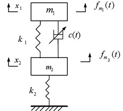
A simplified physical model of the bilinear system is shown in Fig. 1, which is a double-layer vibration suppression bilinear system. The specific parameters of this system are introduced as follows. Where the sprung mass and the unsprung mass , spring and spring , intelligent damper with damping coefficient .
The dynamic equations of the system can be written down as:
where, , , denote, respectively, the displacement, velocity, and acceleration of the sprung mass , , , and are the corresponding ones of the unsprung mass . is a disturbance force acting on the sprung mass . is the output force acting on the unsprung mass . The transfer function can be solved by using Laplace transformation:
The parameter values are given as follows: 138 kg, 125 kg, 26.69×10³ N/m, 129.55×10³ N/m.
Fig. 1Model of double-layer vibration suppression bilinear system
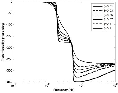
The transfer function of the system can be calculated by Eq. (5), when damping ratio can be taken from different values of 0.01 to 0.2. Fig. 2-3 show the amplitude-frequency response curve (FRC) and phase-FRC of transmissibility, respectively. It can be seen from Fig. 2-3, there are two peak values 2 Hz and 5.7 Hz in the double-layer vibration suppression system, respectively.
Fig. 2Amplitude FRC of transmissibility
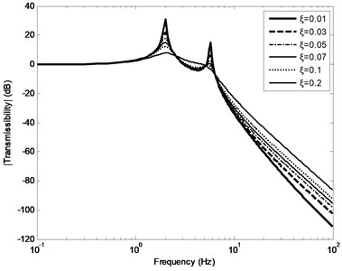
Fig. 3Phase FRC of transmissibility
The state equations of system are established on the basis of a double-layer vibration suppression bilinear system model ahead being created and differential Eqs. (1-2), in the following context, which are used to study the vibration suppression effect of a double-layer vibration suppression under the technology of damping control.
State variables are defined as , , , , choosing the state variables as:
The following state-space Eqs. (7-8) are obtained:
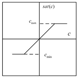
The damper of the double-layer vibration suppression system is a nonlinear element in this paper. The saturation nonlinear of the actuator is of typical characteristics of a semi-active double-layer vibration suppression system, in other words, saturation nonlinear exist in any form of adjustable damper, it has a very important significance to further study the nonlinear control of semi-active double-layer vibration suppression system. The nonlinear saturation is one of the most common nonlinear characteristic of control system. Almost all the actual systems, when signal is large enough to drive, due to that various kinds of components that make up a system are limited by the largest capabilities, will appear as the saturation phenomenon. As shown in Fig. 4 it is an idealized typical nonlinear saturation.
Eq. (9) shows the linearization of nonlinear saturation, c is the controllable yield damping force of the damper. The mathematical expression is:
It can be seen that this system model of double-layer vibration suppression is the bilinear system model from Eqs. (7-9) in this paper.
Fig. 4Nonlinear characteristics of idealized saturation
3. Research of semi-active damping control strategy
The effects of vibration suppression of the semi-active control can be achieved through the real-time adjusting mass, stiffness and damper of the vibration suppression system. In practical application, changing the damping coefficient is relatively easy to implement, and there are more mature approaches such as electro-rheological (ER), magneto-rheological (MR) smart dampers and so on.
3.1. Research of Skyhook damping control strategy
Skyhook damping control strategy was put forward by D. Karnopp [13]. This kind of vibration suppression model was based on a single degree of freedom. In practice, it is not possible to connect the damping with a fixed reference plane, at this time the damping force being provided is proportional to the absolute speed of the mass. This is a kind of ideal condition, called “ceiling” damping, damping coefficient as . Suppose that the speed of incentive input layer is , the speed after vibration suppression is . The actual control algorithm based on the “skyhook damping” is as follows:
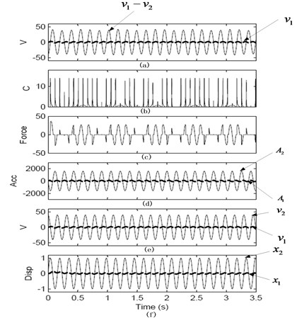
The numerical simulation was performed based on this system under this control strategy. Taking system damping ratio 0.7, the simulation was programmed using Matlab under the condition of the single frequency excitation signal four times of the system natural frequency. The controllable damping value is determined by the Eq. (10). As shown in Fig. 5, the output force switch between zero and skyhook damping force under the condition of high frequency input excitation signals. As shown in Fig. 5, the suppression effects of the semi-active control for speed and displacement peak are obvious, the control effect of high frequency part has been increased significantly.
Fig. 5Steady-state response of skyhook damping semi-active control systems under sine excitation
3.2. Research of ODSAC strategy
Due to the limitations of the passive vibration suppression technology, the effect of vibration suppression under the condition of more complex signal frequency components of the input force is bad, the better effect of vibration suppression technology is needed to be found. The vibration suppression effect can be achieved by means of real-time adjusting the mass, stiffness and damping of the semi-active vibration suppression system. Now more mature methods are used to change the damping coefficient, so far, the methods of changing the damping values of damper have already a lot of ready-made solutions, such as the commonly used ones with electro-rheological and magneto-rheological damper, etc. So the methods of damping coefficient change of semi-active control system are used to achieve the vibration suppression.
3.2.1. The derivation of optimal damping based on generalized variational method
On account of , is constant, so defines the objective function :
where is the displacement of the unsprung mass , and is the initial time and the end time.
Because the damping coefficient of the Eqs. (1-2) is variable, namely, is the function of the time . Namely:
So, now the problem is transformed to solve so as to make minimum.
The optimal control problems described in Eq. (12) are functional conditional extremum problems.
Under the condition of no limit on the value of , the differential Eq. (1-2) of the system are the equality constraints to deal with.
According to the Lagrange multiplier method, introducing the multiplier vector 1 and 2 , unconstrained functional extremum problems can be transformed from these above-mentioned equality constraint functional extremum problems.
Therefore, taking Lagrange function:
So, now the problem becomes:
Now the variational method is used to solve Eq. (14). Classical variational method is based on such basic assumption: the value range of the controlled variable are not subject to any restrictions, namely, the control domain is full of the whole control space, or is an open set.
Here, however, the controlled variable damping is constrained:
Now the classical variational method is powerless.
The generalized variational method, namely Pontryagin’s Maximum Principle is used to solve these problems above.
As shown in Fig. 1, the differential equations are transformed into state space equations by Eq. (6):
The initial state is set to:
According to the condition of the principle of minimum, establishing the Hamilton function is:
Based on the Hamilton principle, the necessary condition that the system obtains extreme value is:
By simplifying the results, the following is obtained:
The conditions of the final value are:
According to the condition of the principle of minimum, seeking the extreme value to be minimal, the parts relate to should be minimum, namely:
should be minimum.
Since it is difficult to work out the Eq. (16) and Eq. (20), let’s study the numerical method approximately solving the damping coefficient c(t).
3.2.2. Theoretical derivation of optimal damping non-differentiable control curve
(1) function:
The function defined in the real domain is called as function which satisfy the following conditions:
When 0, , is an arbitrary function which is continuous at 0.
Due to Eq. (22), can be defined as:
Among above equations, when , 0, is an arbitrary function which is continuous when time .
(2) The definition of variational derivative [43]:
For the inner product space , mapping: : → or , is called as a functional on . If , for , , if exist such that:
namely:
denotes the derivative of at . If you take or . Inner product , the above derivative defined is consistent with the definition of ordinary function, and it is also consistent to generalize to or .
Taking as the generalized function space, then inner product , hence, according to this definition and Eq. (24), we can obtain:
where is dimensionless, it can be transformed into:
Denote , is still the generalized function, its values at are usually written as:
(3) The definition of the functional:
Denote , thus there are:
According to the Eq. (23), there is:
From the Eq. (27), one can get to know:
According to the Eq. (28), there are:
Comparing Eq. (30) with Eq. (29), Eqs. (31-32), one can obtain:
Given the objective function Eq. (11), solving its variation gradient, variational derivative is the most critical item among the results, namely:
Making use of the Eqs. (1-2), solving the variational derivative on the damping , yields:
Among them, is given by Eq. (33), namely , , , , all represent solving first derivative and second derivative of the displacement of the sprung mass m1 and unsprung mass versus time , its numerical solution of the can be worked out using the Eq. (35). Here, the relationship between and is more easily confusing. In fact, both of them all denote time, but the difference is that is a certain point of time, and is a time to traverse. It can be understood that each variable of motion Eqs. (1-2) in each certain time point all has a certain status, while solving variational derivative with respect to in Eq. (35) is equivalent as to add a “tiny perturbation function” on every moment , that is . This is the meaning in physics of Eq. (35). At the same time, due to the introduction of the impulse function it can also be understood in mathematics that the influence of continuous non-differentiable points on the optimum control curve is considered.
Now making use of the gradient descent method to calculate the optimal control curve is described below:
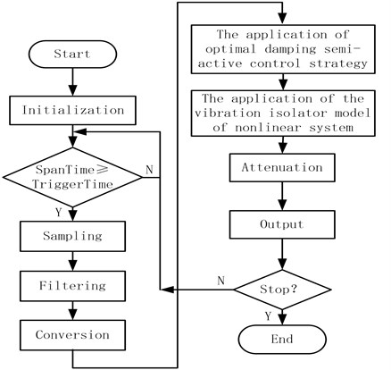
Fig. 6Flow chart of optimal damping solved by using numerical method
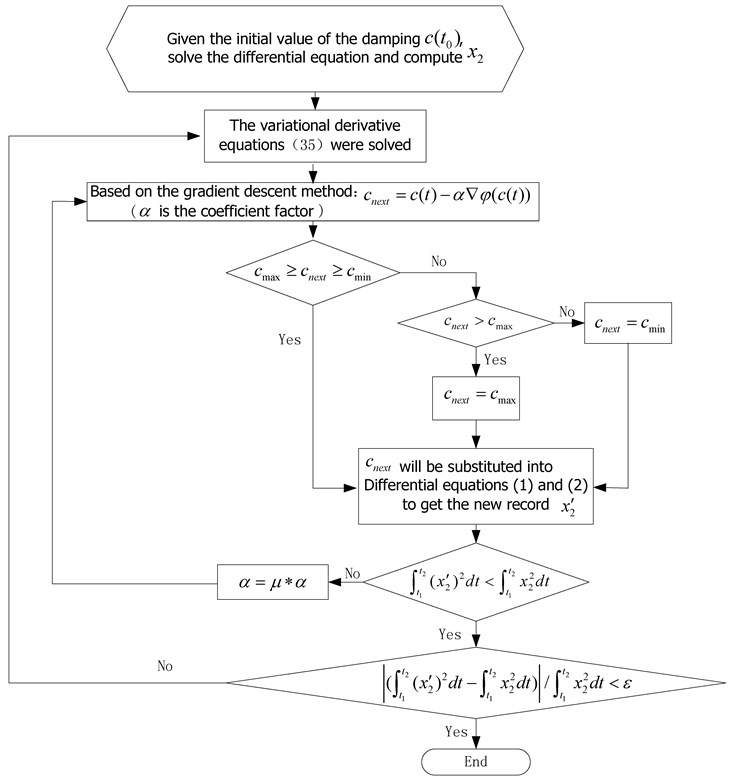
Taking an initial at first, using the optimal passive damping , and then is fixed, and are obtained by numerical solutions of the original problems, and then carrying out numerical solution of Eq. (35), can be got, the gradient direction of can be obtained by substituting into Eq. (35), and then update , the above steps are repeated, until meeting the optimization condition. Fig. 6 shows the flow chart of optimal damping solved by using numerical method. Among in Fig. 6, is the coefficient factor, taking 1013 as the initial value of . is a variable to change , taking 0.7 at first, then adjust parameter values of according to the experimental situation.
3.2.3. Controller stability analysis
The saturation, hysteresis and bilinear characteristic are the main features of strong-nonlinearity model of ERD of double-layer vibration isolation system. The state equation of ERD system dynamics is established as follows:
where is an input variable of the controlled object, namely Electro-rheological controllable yield damping force. is the disturbance input. is the state variables of the system. is the disturbance input matrix. is input matrix. is system matrix:
is the bounded time-varying parameters in ERD vibration isolation system. Time-varying parameter matrix : , , . The stability of the system does not influence the input of the outside world, let the disturbance input is zero (0), then Eq. (36) can be rewritten as follows:
where , , , .
The uncertain systems Eq. (37) are included in the bounded convex polyhedron area which are formations of and “2” vertex matrix of time-varying parameters of the ERD vibration isolation system.
The feedback control rate is as follows:
where is the feedback control matrix [37, 44-46].
Define the Lyapunov function, , . On the basis of the requirements of the theory of stability of the Lyapunov function:
Thus the following equation can be obtained:
where, is additional matrix of feedback, matrix is equal to “0” or “1”. And is the Complementary matrix of , namely , , [37].
The sufficient and necessary condition of Eq. (40) being established is as follows:
Assume that denote domain of attraction, there exists a tiny ellipsoid which is consistent with in structure, this tiny ellipsoid is known as the shape reference set of .
A reference vector is given, is the state space:
Eq. (42) shows that space is compressed times. . When is equal to , shape reference set tend to be , that is the biggest attraction domain.
The feedback controller of the ERD isolation system and namely the biggest attraction domain can be obtained by calculating the optimal solution of the following matrix inequality:
The attraction domain of the closed-loop control system can be described as by the following algebraic equations:
The condition of judging arbitrary system state variables in the attraction domain is the state variables of the system satisfying Eq. (44). So the closed-loop control nonlinear system of the ERD vibration isolation is partial exponential stability in attracting domain.
4. Simulation of vibration suppression control effect and analysis of results
The vibration suppression effect of optimum damping vibration suppression technology was simulated and analyzed by means of observing the cases of output force corresponding to the given input force signal on the basis of the proposed optimization damping control methods ahead.
The output force status will be observed in the case of mixed signals of different input force frequencies, such as impact and sine mixed signals, random and sine mixed signals, random and impact mixed signals. The vibration suppression control effect of the optimized damping control is compared with passive damping control and skyhook damping control. According to the practical engineering experience, in the following simulation, the maximum damping coefficient of the damper is taken as 1609.7 N∙m-1∙s, when is approximately equal to 0.2. While the minimum damping coefficient of the damper is taken as 402.415 N∙m-1∙s, when is approximately equal to 0.05. The optimal passive damping coefficient is called as , when is approximately equal to 0.14, namely 1126.8 N∙m-1∙s. When is approximately equal to 0.15, namely the skyhook damping coefficient as 1207.2 N∙m-1∙s. The given input force is a single frequency sine signal, , where 2Hz.
4.1. Research on vibration suppression effect of impact and sine mixed input signals
The transient system response can generally be ignored under harmonic excitation and periodic excitation force, due to the role of damping. However, in some cases, although the transient process time that the system being suffered by incentives (such as the impact force or the machine running a mutation) is very short, but the vibration amplitude is great, the phenomenon of the short-term overstressing will be produced in some parts inside the machine, these have greater destructive power. Therefore, the study of transient impact incentive signal is very necessary.
In the actual project, the frequency components included in input force are more complex. Now more common case of input force for impact and sine mixed signal will be simulated in the following context.
A given input force is an impact and sine mixed signal input force. The impact force can be expressed as follows:
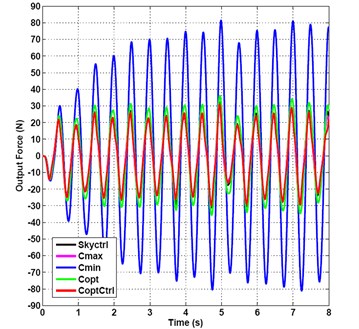
It can be seen from Fig. 7 that the output force time domain curves obtained by semi-active optimal damping control compared to several other control curves are more “smooth”, that is to say, under the impact and sine mixed signal input, the effects of optimal control damping are better, so the best effects of vibration suppression can be gotten. Fig. 7 also shows that the amplitude of the minimum damping vibration suppression control are increasing from small to large, reaching the maximum 77 N to the steady status after four seconds, while the effects of the semi-active optimal damping vibration suppression are better than the other four control methods.
Although five control methods all have not obvious isolation effects, but the amplitudes of the semi-active optimal damping vibration suppression are smaller than that of the other four curves, the “overshoot” of semi-active optimal damping vibration suppression is relatively smaller, so the best comprehensive performance indexes can be obtained.
The frequency-spectrum graph of the five kinds of damping control methods is shown in Fig. 8. The first-order and second-order natural frequencies of vibration suppression system are close to 2 and 5.7 Hz. The frequency-spectrum value of the minimum passive damping vibration suppression is 16.69 dB at resonance frequency of 2 Hz, it is the largest frequency-spectrum value of the five kinds of damping control methods. The frequency-spectrum value varied sharply to –23.92 dB at frequency 5.75 Hz. The frequency-spectrum value of the optimal damping semi-active control arrives to its maximum peak value 7.07 dB at frequency of 2 Hz, it is the smallest frequency-spectrum value of the five kinds of damping control methods at frequency of 2 Hz. And then the value reaches the local minimum of –41.11 dB at frequency of 5.12 Hz, go to –35.09 dB at frequency of 5.75 Hz, and then to the second peak value –7.63 dB at frequency of 6 Hz.
The optimal control damping of output force is shown in Fig. 9. This illustrates that the damping values change from starting point 1610, then drop to minimum value point 402.4 from 0.2 seconds, then to the maximum value point 1610 again, and then period circle at the intervals of every 0.2 seconds. So we can take either maximum damping control at the origin point or minimum damping control after every almost 0.2 second time period, and then run in accordance with period circles.
Fig. 7Output force under impact and sine mix signal incentive
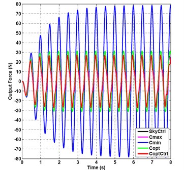
Fig. 8Frequency-spectrum graph of output force under impact and sine mix signal incentive
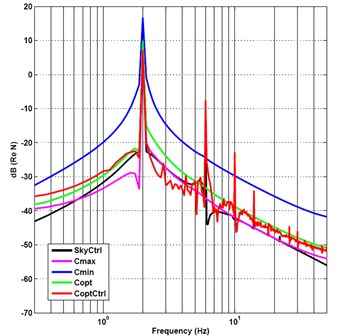
Fig. 9Optimal control damping of output force under impact and sine mixed signals incentive
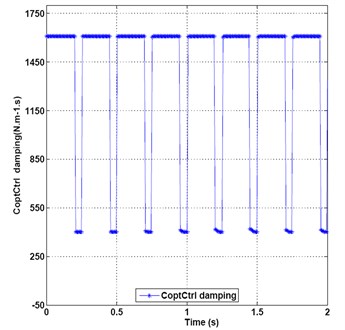
Fig. 10Output force under random and sine mix signal incentive
4.2. Research on isolation effect of random and sine mix input signal
Now more common case of input force for random and sine mixed signal will be simulated in the following context. Now a given input power is a uniform distribution random signal and sine mixed signal, the maximum amplitude is 10.
Due to the vibration suppression system is mainly used in the mechanical system; the limit of general mechanical system vibration frequency is 50 Hz, so that the frequency range was chosen as 0.1 to 50 Hz. Because of the frequency components of the random signal are as much as all frequency components, including the frequency components after 50 Hz, so a low pass filter is needed to add, filtering out the frequency components of a random signal after 50 Hz.
It can be seen from Fig. 10 that the amplitude of the output force time domain curves obtained by semi-active optimal damping control compared to several other control curves is the smallest, so that the best effects of vibration suppression can be gotten under the random and sine mixed input signal.
The amplitude of the minimum damping control vibration suppression is shown in Fig. 10, it is increasing from 28.43 to 70.39, reaching the local maximum 80 N to the relatively steady status after 4.5 seconds.
The frequency-spectrum graph of the five kinds of damping control methods is shown in Fig. 11. The frequency-spectrum value of the minimum passive damping vibration suppression is 16.33 dB at resonance frequency of 2Hz and the frequency-spectrum value varied sharply to –23.56 dB at 5.7 Hz. The frequency-spectrum value of the optimal damping semi-active control reaches 6.76 dB in its maximum peak value at 2 Hz, it is also the most smallest frequency-spectrum value of the five kinds of damping control methods at frequency 2 Hz. And then it is passing the local minimum –38 dB at 5.87 Hz, and then to the second peak value –12.54 dB at 6 Hz. So the frequency spectrum characteristic of the optimal damping control is the best of the five kinds of control methods at the first-order and second-order natural frequencies.
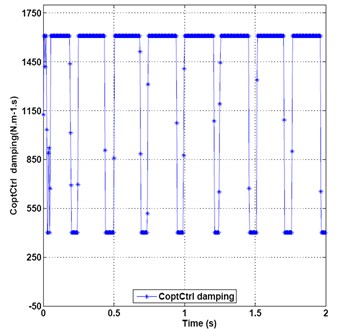
Fig. 12 shows the optimal control damping of output force. This illustrates that the damping values change from starting point 1127, then rise to 1610, persist 1610 for 0.15 seconds, then drop to middle transition value point 1437, 1015, 693, 402, then rise up to 1610, persist for 0.2 seconds, then drop down to 402.4 from 0.44 second, then to maximum value point 1610 again, and then repeat period circle at the intervals of every 0.2 seconds. So the maximum damping control can mainly be taken and minimum damping control can be adopted in smaller portions.
Fig. 11Frequency-spectrum graph of output force under random and sine mix signal incentive
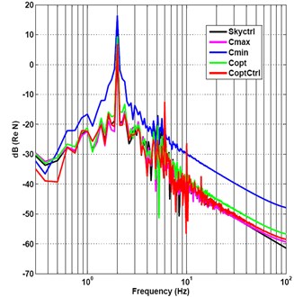
Fig. 12Optimal control damping of output force under random and sine mixed signals incentive
4.3. Research on isolation effect of random and impact mix input signal
Now the random and pulse input force mixed signal will be simulated in the following context. Now a given input power is a uniform distribution random signal and pulse mixed signal, the maximum amplitude is 10.
It can be seen from Fig. 13 that the amplitude of the output force time domain curves obtained by semi-active optimal damping control compared to several other control curves is the smallest, that is to say, under the random and impact mixed input signal, the best effects of vibration suppression can be gotten. Fig. 13 shows that the amplitude of the skyhook damping vibration suppression is the biggest, its overshoot is obvious, while the amplitude of the semi-active optimal damping vibration suppression is smaller than the other four control methods. Five control methods all have obvious effects of vibration suppression.
The frequency-spectrum graph of five damping control methods is shown in Fig. 14. The frequency-spectrum value of the minimum passive damping vibration suppression is –11.42 dB, namely the maximum value of five control methods at a resonance frequency of 2 Hz and the frequency-spectrum value varied sharply to –22.12 dB at 5.7 Hz. The frequency-spectrum value of the optimal semi-active control damping reaches –19.49 dB at 2 Hz, namely the minimum frequency spectrum value of five control methods and the local minimum of –44.33 dB at 3.38 Hz then to the value –30.23 dB at 5.75 Hz.
The optimal control damping of the output force is shown in Fig. 15. This illustrates that the damping values change from starting point 1610, then drop to middle transition value point 1192, then rise up to 1610, then drop down to minimum value 402.4 from 0.08 seconds, then to maximum value point 1610 again, and then oscillating during 0.2 seconds, the percentages of the maximum damping values are much more than the percentages of the minimum damping values.
So we can take mainly maximum damping control and a small part of minimum damping control according to the curves of damping control.
Fig. 13Output force under random and impact mix signal incentive
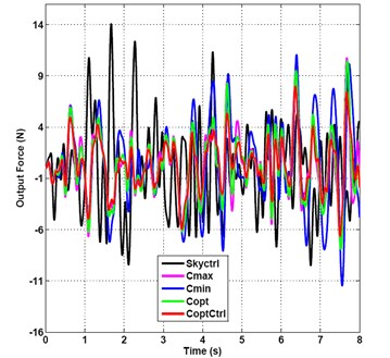
Fig. 14Frequency-spectrum graph of output force under random and impact mix signal incentive
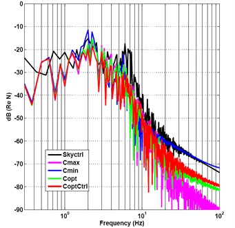
Fig. 15Optimal control damping of output force under impact and random mixed signals incentive
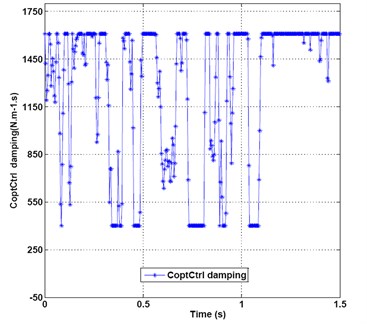
Table 1RMS value of output force of five kinds of damping control effects under three kinds of mixed signal incentive (N)
Three kinds of input excitation signals | Five kinds of damping control methods | ||||
Maximum passive damping | Minimum passive damping | Optimal passive damping | Skyhook damping | Optimal semi-active damping | |
Impact and sine mixed signals | 16.85 | 49.82 | 21.45 | 17.16 | 16.36 |
Random and sine mixed signals | 16.49 | 48.09 | 20.88 | 17.06 | 15.83 |
Random and impact mixed signals | 3.02 | 4.08 | 3.10 | 4.10 | 2.44 |
The exact root mean square (RMS) values of the output force of the five kinds of damping control methods under impact and sine mixed signals, random and sine mixed signals, and random and impact mixed signals incentive are listed in Table 1. The isolation effect of optimum semi-active damping is superior to that of the minimum passive damping isolation and that of the optimal passive damping, it is close to that of the maximum passive damping vibration suppression and the skyhook damping control vibration suppression, so that the isolation effect of the semi-active optimal damping control is the best of the five kinds of damping control strategies under three kinds of mixed input signal incentive. The vibration suppression effect of the impact and random mixed input signals is remarkable.
5. Experiment
5.1. Experimental equipment
The experiment of the double-layer vibration isolation of bilinear system was proceeded in the Institute of Intelligent Mechatronics Research (IIMR) of Shanghai Jiao Tong University. The main equipments used in the experiments are that the Pulse analyzer of Denmark B&K company, ten piezoelectric type acceleration sensors of B&K, Charge amplifier, Sony digital signal recorder, two electro-magnetic vibrators for modal analysis, two PCB modal force hammers, four PCB micro ICP acceleration sensors, double-layer vibration isolation experiment platform, and so on.
The ERF damper with single damping duct developed by our laboratory is shown in Fig. 16.
Fig. 16ERF damper with single damping duct
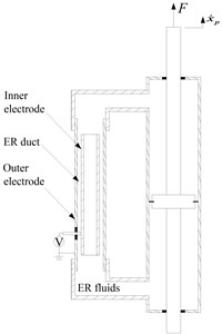
a) Schematic configuration
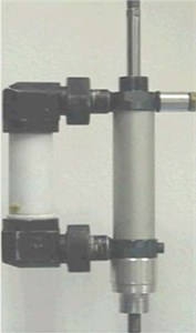
b) Photograph
5.2. Properties of ERF damper
The schematic diagram of the bypass ERF damper with single damping duct used in this study is shown in Fig. 16. The damper consists of a hydraulic cylinder, which is divided into two working chambers by a piston. The bypass, fitted to the side of the hydraulic cylinder, comprises two concentric tubular electrodes and an annulus through which the ER fluids flow. The positive voltage produced by a high voltage supply unit is applied to the inner electrode, while the negative voltage is connected to the outer electrode. In defect of electric fields, the ERF damper produces the viscous damping force only by the fluid-flowing resistance. However, if a certain level of the electric voltage is supplied to the ERF damper, additional damping force due to the yield stress of the ER fluid would be produced. This damping force of the ERF damper can be continuously tuned by changing the voltage applied to the damper. Based on the Bingham constitutive model of ER fluids, which is sufficiently accurate for design calculation although it does not capture details of the deformation behavior of an actual damper, the approximation of the damping force in the bypass damper is obtained as follows:
where:
where is no-applied voltage damping coefficient, which is determined by the plastic viscosity of ER fluids and the geometry of the manufactured damper, is the controllable yield stress damping force generated by the applied voltage, , and are the intrinsic parameters of the ERF damper and can be experimentally determined, is the voltage; is the velocity of piston motion, and is a signum function.
Fig. 17 reports the measured damping force with respect to the piston velocity at various voltages. It is obtained by calculating the maximum damping force at each velocity. The piston velocity increases from 15 to 100 mm/s gradually, while the excitation amplitude is maintained to be constant at 60 mm. Such a plot is frequently employed to evaluate the level of damping performance in the damper manufacturing industry. For the proposed damper with single damping duct the damping force increased with the applied voltage, as expected. For instance, the damping force increases up to 227 N at a piston velocity of 100 mm/s and voltage of 5 kV. This Figure agrees fairly well with the presented damping model given by Eq. (46).
Chart of real-time controlling module is shown in Fig. 18.
Fig. 17Under various voltages damping force of ERF damper with single damping duct versus piston velocity, U= 0.0 kV (dot line), U= 1.4 kV (dash dot line), U= 2.5 kV (dash line), U= 3.5 kV (solid line), and U= 5.0 kV (thick line)
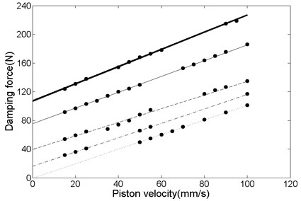
Fig. 18Chart of real-time controlling module
5.3. Measurement experiment of transmissibility and result analysis under condition of no vibration isolator
The vibrator working at a fixed frequency is used in the measuring experiments. The parameters of the force vibration isolation testing bench are as follows:
The sprung mass 60 kg, the unsprung mass 16 kg, the stiffness of the sprung mass 33000 N/m, the stiffness of the unsprung mass 185000 N/m. The undamped force transfer rate of this test bed can be calculated according to the theoretical formula, the transmissibility curve is shown in solid line of Fig. 19. When the ERF vibration isolator is not installed in a force vibration isolation test-bed, the measured force transmissibility curve of the double layer vibration isolation (square icon shown in Fig. 19) is consistent with the theoretical curve; this illustrate that the measurement method is reliable. As shown in Fig. 19, the first and the second-order natural frequency of the vibration isolation system is 3.4 Hz and 18.64 Hz, respectively. The maximum transmissibility of the first-order and the second-order system are 57 and 38.71, respectively.
Fig. 19Transmissibility of double-layer force isolation testing bench with no damper
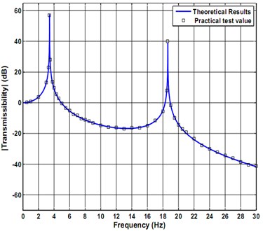
Fig. 20Force transmissibility of double-layer vibration suppression bilinear system with ODSAC law with single damping orifice ERD
5.4. Experiment of ERF damper with single damping orifice under ODSAC of double layer vibration isolation bilinear system
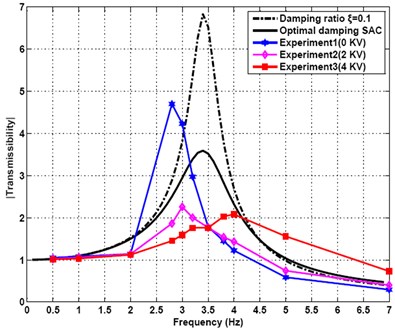
In order to further validate the control effect of actual vibration isolation of bilinear system under the action of the ODSAC which is designed in this paper, the experiment of ERF damper with single damping duct is carried out in the above experiment platform of the force vibration isolation system. Where 10.23 N, 6.38 N/kV, 2.59 N/kV2, no-applied voltage viscous damping coefficient 1013.4 N∙m-1∙s. The sampling frequency of a randomly profiled roadway input excitation is 300 Hz. The signal frequency is 2 Hz, 2.8 Hz, 3 Hz, 3.2 Hz, 3.5 Hz, 3.8 Hz, 4 Hz, 5 Hz, 7 Hz, respectively. The transmissibility of double-layer vibration isolation bilinear system under different frequency randomly profiled roadway input excitation signals at a different voltage are listed in Table 2. The frequency domain curve of the transmissibility of the system can be drawn from this data, which is shown in Fig. 20. It can be seen from the diagram that the first order resonance peak frequency of the practical system is about 2.8 Hz, the vibration amplitude of the upper quality is the largest in here. It is observed that the first order resonant frequency of the actual system is different from the theoretical calculation value, this is because that the quality itself of spring and damper of the actual system will affect the vibration isolation system. The different voltages (0 KV, 2 KV, 4 KV) being applied in ERF damper in the resonance peak play an obviously different vibration reducing effects. The greater the applied voltage is, the lower the transmissibility is. This is completely consistent with the theoretical analysis.
It can also be seen from the Fig. 20 that the applied voltage can make the transmissibility increase instead when the excitation frequency is greater than 3.5 Hz, namely the crossover frequency of system. The transmissibility curve of the passive damping control of vibration isolation as damping ratio 0.1 and the optimal damping semi-active control (ODSAC) of vibration isolation can be seen from Fig. 20.
The results show that the vibration isolation effect of the double-stage force vibration isolation bilinear system under the action of the ODSAC is better than that of the passive damping vibration isolation control system. Although there are some deviations, compared with the results of experimental test, but the trend is consistent with the measured transmissibility curve, this shows that the proposed control method is feasible and effective.
Table 2Transmissibility of double-layer vibration isolation bilinear system using different voltages under signal excitation of randomly profiled roadway input
Voltages/ Transmissibility/ Frequency | 2 Hz | 2.8 Hz | 3 Hz | 3.2 Hz | 3.5 Hz | 3.8 Hz | 4 Hz | 5 Hz | 7 Hz |
0 KV | 1.142 | 4.700 | 4.230 | 2.971 | 1.783 | 1.448 | 1.222 | 0.586 | 0.293 |
2 KV | 1.135 | 1.863 | 2.257 | 2.001 | 1.766 | 1.538 | 1.431 | 0.741 | 0.398 |
4 KV | 1.120 | 1.453 | 1.599 | 1.759 | 1.762 | 2.037 | 2.088 | 1.558 | 0.730 |
5.5. Experiment of ERF damper under recorded signal of randomly profiled roadway input excitation
It can be seen from Fig. 21 that the amplitude of the output force time domain curves obtained by ODSAC compared to several other control curves is the smallest, so that the best effects of vibration suppression can be gotten under a recorded signal of a randomly profiled roadway input excitation.
Fig. 21Output force under recorded signal of randomly profiled roadway input excitation
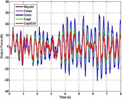
Fig. 22Frequency-spectrum graph of output force under recorded signal of randomly profiled roadway input excitation
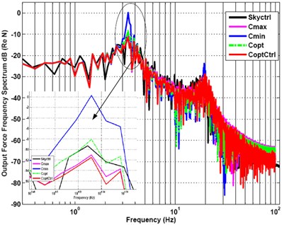
The frequency-spectrum graph of the five kinds of damping control methods is shown in Fig. 22. The frequency-spectrum value of the minimum passive damping vibration suppression is 0.26 dB at resonance frequency of 3.4 Hz, and the frequency-spectrum value varied sharply to –23.66 dB at 19.5 Hz. The frequency-spectrum value of ODSAC arrive at –11.48 dB in its maximum peak value at 3.4 Hz, it is also the smallest frequency-spectrum value of the five kinds of damping control methods at frequency 3.4 Hz. And then it is passing to the local minimum of –49.08 dB at 19.3 Hz. So the frequency spectrum characteristic of ODSAC is the best of the five kinds of control methods at the first-order and second-order natural frequencies.
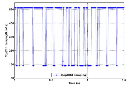
Fig. 23 shows the optimal control damping of output force. This illustrates that the damping values change from starting point 562.8, then drop to minimum value point 140.7, then to maximum value point 562.8 again, and then repeat period circle.
Fig. 23Optimal control damping of output force under recorded signal of randomly profiled roadway input excitation
The exact RMS values of the output force of the five kinds of damping control methods under a recorded signal of randomly profiled roadway input excitation are listed in Table 3. The isolation effect of ODSAC is much better than that of the minimum passive damping isolation and that of the optimal passive damping, so that the isolation effect of the ODSAC is the best of the five kinds of damping control strategies under a recorded signal of a randomly profiled roadway input excitation.
Table 3RMS value of the output force of five kinds of damping control effects under recorded signal of randomly profiled roadway input excitation (N)
Input excitation signals | Five kinds of damping control methods | ||||
Maximum passive damping | Minimum passive damping | Optimal Passive damping | Skyhook damping | Optimal semi-active damping | |
Recorded signal of randomly profiled roadway input excitation | 6.05 | 11.99 | 7.00 | 6.44 | 5.89 |
6. Conclusions
This study successfully demonstrates the application of a optimal damping semi-active control strategy to a double-layer vibration suppression bilinear system which is subjected to the mix signal of single-frequency sine and pulse input signal, the mix signal of random and sine signal, the mix signal of random and impact input signal. Five control algorithms have been studied, which are based on semi-active optimal damping control, skyhook damping control, and passive damping control. Using the model of vibration suppression bilinear system, the vibration suppression performance of the optimal damping control algorithms has been analyzed and compared with that of the passive one and the skyhook damping controls methods. It can be concluded from the results of the ERF experiments and simulations that the optimal damping semi-active control methods considered can provide much better effects of vibration suppression under three mixed signal than that of a conventional passive damping and skyhook damping control. The isolation effects of the optimal damping semi-active control are the best of the five kinds of damping control methods, and the vibration reduction effect of the random and shock input mixed signal is prominent. The relation of the optimal damping semi-active control, skyhook damping control and balance control need to be deeply studied. The control method of bilinear model linearization will be deeply studied in future.
References
-
Cai L. B., Chen D. Y. A two-stage vibration isolation system featuring an electrorheological damper via the semi-active static output feedback variable structure control method. Journal of Vibration and Control, Vol. 10, Issue 5, 2004, p. 683-706.
-
Chen X., Qi H., Zhang Y., Wu C. Optimal design of a two-stage mounting isolation system by the maximum entropy approach. Journal of Sound and Vibration, Vol. 243, Issue 4, 2001, p. 591-599.
-
Royston T., Singh R. Optimization of passive and active non-linear vibration mounting systems based on vibratory power transmission. Journal of Sound and Vibration, Vol. 194, Issue 3, 1996, p. 295-316.
-
Sun T., Huang Z., Chen D. Signal frequency-based semi-active fuzzy control for two-stage vibration isolation system. Journal of Sound and Vibration, Vol. 280, Issues 3-5, 2005, p. 965-981.
-
Jayachandran R., Krishnapillai S. Modeling and optimization of passive and semi-active suspension systems for passenger cars to improve ride comfort and isolate engine vibration. Journal of Vibration and Control, Vol. 19, Issue 10, 2013, p. 1471-1479.
-
Ghosh M. K., Dinavahi R. Vibration analysis of a vehicle system supported on a damper-controlled variable-spring-stiffness suspension. Proceedings of the Institution of Mechanical Engineers, Part D – Journal of Automobile Engineering, Vol. 219, Issue 5, 2005, p. 607-619.
-
Issa J. S. Ground motion isolation using a newly designed vibration absorber. Proceedings of the Institution of Mechanical Engineers, Part C – Journal of Mechanical Engineering Science, Vol. 226, Issue 3, 2012, p. 636-647.
-
Zhao W., Li B., Liu P., Liu K. F. Semi-active control for a multi-dimensional vibration isolator with parallel mechanism. Journal of Vibration and Control, Vol. 19, Issue 6, 2013, p. 879-888.
-
Ying Z. G., Zhu W. Q. A stochastic optimal semi-active control strategy for ER/MR dampers. Journal of Sound and Vibration, Vol. 259, Issue 1, 2003, p. 45-62.
-
Ji H., Qiu J., Nie H., Cheng L. Semi-active vibration control of an aircraft panel using synchronized switch damping method. International Journal of Applied Electromagnetics and Mechanics, Vol. 46, Issue 4, 2014, p. 879-893.
-
Liu Y., Waters T. P., Brennan M. J. A comparison of semi-active damping control strategies for vibration isolation of harmonic disturbances. Journal of Sound and Vibration, Vol. 280, Issues 1-2, 2005, p. 21-39.
-
Hiramoto K., Matsuoka T., Sunakoda K. Simultaneous optimal design of the structural model for the semi-active control design and the model-based semi-active control. Structural Control and Health Monitoring, Vol. 21, Issue 4, 2014, p. 522-541.
-
Karnopp D., Crosby M., Harwood R. Vibration control using semi-active force generators. ASME Journal of Engineering for Industry, Vol. 96, Issue 2, 1974, p. 619-626.
-
Rakheja S., Sankar S. Vibration and shock isolation performance of a semi-active ‘on-off’ damper. ASME, Transactions, Journal of Vibration, Acoustics, Stress, and Reliability in Design, Vol. 107, Issue 4, 1985, p. 398-403.
-
Alanoly J., Sankar S. A new concept in semi-active vibration isolation. Journal of Mechanisms, Transmissions, and Automation in Design, Vol. 109, Issue 2, 1987, p. 242-247.
-
Cheok K. C., Loh N. K., McGee H. D., Petit T. F. Optimal model-following suspension with microcomputerized damping. IEEE Transactions on Industrial Electronics, Vol. 32, Issue 4, 1985, p. 364-371.
-
Tseng H., Hedrick J. Semi-active control laws-optimal and sub-optimal. Vehicle System Dynamics, Vol. 23, Issue 1, 1994, p. 545-569.
-
Hrovat D., Margolis D., Hubbard M. An approach toward the optimal semi-active suspension. Journal of Dynamic Systems, Measurement, and Control, Vol. 110, Issue 9, 1988, p. 288-296.
-
Hrovat D. Survey of advanced suspension developments and related optimal control applications. Automatica, Vol. 33, Issue 10, 1997, p. 1781-1817.
-
Ho C., Lang Z. Q., Sapinski B., Billings S. A. Vibration isolation using nonlinear damping implemented by a feedback-controlled MR damper. Smart Materials and Structures, Vol. 22, Issue 10, 2013, p. 1-11.
-
Peng Z. K., Lang Z. Q., Jing X. J., Billings S. A., Tomlinson G. R., Guo L. Z. The transmissibility of vibration isolators with a nonlinear antisymmetric damping characteristic. Journal of Vibration and Acoustics – Transactions of the ASME, Vol. 132, Issue 1, 2010, p. 1-7.
-
Soliman J., Ismailzadeh E. Optimization of unidirectional viscous damped vibration isolation system. Journal of Sound and Vibration, Vol. 36, Issue 4, 1974, p. 527-539.
-
Zhao C., Chen L., Chen D. Y. Semi-active static output feedback variable structure control for two-stage vibration isolation system. Journal of Vibration and Acoustics-Transactions of the ASME, Vol. 128, Issue 5, 2006, p. 627-634.
-
Zhao C., Chen D. Y. A two-stage floating raft isolation system featuring electrorheological damper with semi-active fuzzy sliding mode control. Journal of Intelligent Material Systems and Structures, Vol. 19, Issue 9, 2008, p. 1041-1051.
-
Zhao C., Chen D. Y. A Two-stage floating raft isolation system featuring electrorheological damper with semi-active static output feedback variable structure control. Journal of Intelligent Material Systems and Structures, Vol. 21, Issue 4, 2010, p. 387-399.
-
Okubo H., Yano H., Itoh T. Semi-active vibration suppression for smart structures with sliding-mode control. Journal of Intelligent Material Systems and Structures, Vol. 25, Issue 7, 2014, p. 865-870.
-
Gao X., Chen Q. Theoretical analysis and numerical simulation of resonances and stability of a piecewise linear-nonlinear vibration isolation system. Shock and Vibration, 2014, p. 1-12.
-
Harvey P. S., Gavin H. P., Scruggs J. T. Optimal performance of constrained control systems. Smart Materials and Structures, Vol. 21, Issue 8, 2012, p. 085001.
-
Anh N. D., Nguyen N. Design of non-traditional dynamic vibration absorber for damped linear structures. Proceedings of the Institution of Mechanical Engineers, Part C – Journal of Mechanical Engineering Science, Vol. 228, Issue 1, 2014, p. 45-55.
-
Potter J. N., Neild S. A., Wagg D. J. Generalisation and optimisation of semi-active, on-off switching controllers for single degree-of-freedom systems. Journal of Sound and Vibration, Vol. 329, Issue 13, 2010, p. 2450-2462.
-
Liang J. R., Liao W. H. Piezoelectric energy harvesting and dissipation on structural damping. Journal of Intelligent Material Systems and Structures, Vol. 20, Issue 5, 2009, p. 515-527.
-
Feng J., Ying Z. G., Zhu W. Q., Wang Y. A minimax stochastic optimal semi-active control strategy for uncertain quasi-integrable Hamiltonian systems using magneto-rheological dampers. Journal of Vibration and Control, Vol. 18, Issue 13, 2012, p. 1986-1995.
-
Ledezma-Ramirez D. F., Ferguson N. S., Brennan M. J. Shock isolation using an isolator with switchable stiffness. Journal of Sound and Vibration, Vol. 330, Issue 5, 2011, p. 868-882.
-
Newell D. B., Richman S. J., Nelson P. G., Stebbins R. T., Bender P. L., Faller J. E., Mason J. An ultra-low-noise, low-frequency, six degrees of freedom active vibration isolator. Review of Scientific Instruments, Vol. 68, Issue 8, 1997, p. 3211-3219.
-
El Beheiry E. M. A method for preview vibration control of systems having forcing inputs and rapidly-switched dampers. Journal of Sound and Vibration, Vol. 214, Issue 2, 1998, p. 269-283.
-
Lin Z., Lv L. Set invariance conditions for singular linear systems subject to actuator saturation. IEEE Transactions on Automatic Control, Vol. 52, Issue 12, 2007, p. 2351-2355.
-
Hu T., Lin Z., Chen B. M. Analysis and design for discrete-time linear systems subject to actuator saturation. Systems and Control Letters, Vol. 45, Issue 2, 2002, p. 97-112.
-
Hu T., Lin Z., Chen B. M. An analysis and design method for linear systems subject to actuator saturation and disturbance. Automatica, Vol. 38, Issue 2, 2002, p. 351-359.
-
Yue Y. H., Wang M., Zhao Q. The design of feedback controller for the suspension system with saturated uncertain magneto-rheological damper. Automotive Engineering, Vol. 34, Issue 7, 2012, p. 613-617.
-
Gao X. K., Shao H. Semi-active optimal control of intelligent damping double-deck vibration isolation system. Journal of Vibration and Shock, Vol. 31, Issue 19, 2012, p. 128-133.
-
Gao X. K. Optimal semi-active damping control of the ship raft vibration reduction bilinear system. Journal of Vibration and Shock, Vol. 31, Issue 20, 2012, p. 131-136.
-
Gao X. K., Fan G. L. Semi-active optimal damping control of double-deck vibration isolation nonlinear system. Proceedings of the 23rd International Conference on Adaptive Structures and Technologies, 2012, p. 115-127.
-
Liberzon D. Calculus of Variations and Optimal Control Theory: A Concise Introduction. Princeton University Press, New Jersey, USA, 2012.
-
Du H., Zhang N., Naghdy F. Actuator saturation control of uncertain structures with input time delay. Journal of Sound and Vibration, Vol. 330, Issues 18-19, 2011, p. 4399-4412.
-
Zhou B., Zheng W. X., Duan G. R. Stability and stabilization of discrete-time periodic linear systems with actuator saturation. Automatica, Vol. 48, Issue 7, 2011, p. 1813-1820.
-
Cao Y. Y., Lin Z. Stability analysis of discrete-time systems with actuator saturation by a saturation-dependent Lyapunov function. Automatica, Vol. 39, Issue 7, 2003, p. 1235-1241.
About this article

This work was supported by the Shanghai Jiao Tong University Innovation Fund for Postgraduates under Grant No. AE030202. Henan Tackle Key Problem of Science and Technology under Grant (No. 102102210454). The Foundation of Education Committee of Henan Province under Grant (No. 2011B520028). The Cultivated Funded Project of Luoyang Normal College under Grant (No. 10000859).
