Numerical study on the aerodynamic noise characteristics of CRH2 high-speed trains

1. Introduction

With the increase of the running speed, the aerodynamic performance of high-speed trains has obviously increased. Researches show that aerodynamic drag takes up about 75 % of total drag when the high-speed train runs at the speed of 200 km/h-300 km/h [1, 2]. The train speed will increase aerodynamic drag. In the meanwhile, aerodynamic noises will be more obvious. When the train runs at the speed of 300 km/h, aerodynamic noises caused by the running train will be more than wheel-rail noises and become the main noise of high-speed trains [3]. In addition, the intensity of aerodynamic noises is in direct proportion to the 6th power of speed [3-5]. The speed of high-speed trains in some routes has reached up to 350 km/h. The aerodynamic noise of high-speed trains causes interior noise pollution, reduces the comfort of passengers [6, 7] and causes very serious noise pollution along railway lines. Europe and Japan have conducted in-depth studies on noise problems at the early stage of high-speed trains and stipulated that the sound pressure level of the position which is 25 m away from the center line of track should not be more than 93 dBA when high-speed trains run at the speed of 300 km/h [8]. Aerodynamic noises are caused by gas flowing through structures or structural motion in fluids. The production and propagation of aerodynamic noises and interaction with structures have developed into the sub-discipline of fluid mechanics [9]. At present, the numerical computation of aerodynamic noises generally takes Lighthill acoustic analogy method as the theoretical basis. In actual computation, firstly, the fluctuation pressure of fluid flowing through structure surface is computed to obtain the right end item of Lighthill equation and FW-H equation is then used to compute far-field aerodynamic noises [3, 10]. Secondly, the aerodynamic noise source of structural surface is computed, namely analyzing the intensity of aerodynamic noise source produced on structure surface [11, 12]. The basic theories of computing aerodynamic noise have been relatively mature. Some common software has integrated strong ability in computing aerodynamic noise. However, it is necessary to constantly conduct in-depth engineering application research on applying the basic theories to high-speed trains and reducing the aerodynamic noise of high-speed trains.

Currently, researches on the aerodynamic noise of high-speed trains mainly include two kinds of methods, namely experimental method and numerical simulation method. In the aspect of experimental research, main experimental method contains wind tunnel test and line test method. It is extremely difficult to uniformly study and verify the correctness of computational model as real train test takes a long time, invests a lot of power-man and material resources and is subject to local actual conditions and noise will be increasingly larger with the increase of operation mileage of the train. Wind tunnel test based on scale model has to satisfy strict test conditions and the numerical matching of scale model and original model. On the other hand, numerical simulation has started to be used by people to predict noises with the development of computer technology. Compared with the test method, numerical simulation is equipped with strong controllability and short computation period and able to concisely compute noises and predict noises under different incoming flow conditions and parameters, especially some working conditions hard to operate in reality. Zhu [13-15] predicted the flow field characteristics of simplified bogies with 1:10 scaling only including wheel-sets and frame structure and the distribution rule of dipoles based on delayed detached eddy simulation (DDES) and FW-H method and verified the correctness of numerical simulation through wind tunnel test. Results showed that the aerodynamic noise of bogies was a broadband noise and there was main single-frequency noise. The frequency of bogies on the first top was mainly caused by vortex shedding. The principal axis of the second dominant frequency interacted with wheels. In addition, the frequency of bogies on the first order was related to the lift of bogies while the frequency of bogies on the second order had nothing to do with the drag of bogies. Wakabayashi [16] used the line test method to test the noise of high-speed trains, and results showed that the noise of the high-speed train in the bogie area decreased by about 1 dB compared with that of E2-1000 high-speed train [17]. Huang [18] established an analysis model for the aerodynamic noise of bogies, focused on studying the aerodynamic noise of bogies as noise sources, and analyzed the effect of bogies on reducing radiation noises at both sides with using skirt plates. Zhang [19] numerically studied the aerodynamic noise of bogies of trailer trains and found that the far-field aerodynamic noise of bogies was a broadband noise and had an obvious directivity, amplitude characteristics and so on. Xiao [20] found the cross-section shape of optimized insulator was an oval through conducting numerical computation for different cross-section shapes of pantograph insulator. In addition, the long axis of the oval should be consistent with the flow direction of airflow. Yu [21] designed 4 kinds of air deflectors and numerically simulated pantographs to find that the noise reduction effect was obvious and sound pressure level decreased by about 3dB after an air deflector was adopted. King [22] adopted dipole source to describe the aerodynamic noise caused by the vortex shedding of pantographs and found that the far-field aerodynamic noise of pantographs was approximately linear to the logarithm of train speed. Noger [23] tested the aerodynamic noise source of pantographs in a low-noise wind tunnel and found that the vertical plane at the back of pantographs was a very important noise source. Sueki [24] adopted porous materials on the pantograph of high-speed trains and obtained the following findings through wind tunnel test. When pantographs ran at the speed of 360 km/h, noise reduced by 1.9 dBA; the amplitude decreased by 5 dBA at 250 Hz in one-third octave; material properties had a great impact on the aerodynamic noise of pantographs; noise reduction effect was obvious. Lee [25, 26] obtained the shape of a low-noise pantograph and the noise reduction effect of a new-type pantograph through optimizing the structure and shape of pantograph head, adopting the low-noise pantograph and conducting wind tunnel test. Liu [27] established a mathematical model for the three-dimensional flow field of head train of high-speed trains, used Lighthill acoustic analogy theory to compute the far-field aerodynamic noise, and applied a broadband noise source model to compute the aerodynamic noise source on the surface of head train. Yamazaki [28] found that train connections were also the main noise sources of high-speed trains through conducting wind tunnel test and real train test.

Based on the above investigation, this paper mainly analyzed the flow field and far-field aerodynamic noise characteristics of the complete train and studied the contribution to main aerodynamic noise sources. When the numerical computation was conducted, this paper considered the aerodynamic model of high-speed trains with bogies and established a computational model for the aerodynamic noise of the complete train with 3-train formation and 6 bogies. In addition, this paper adopted FW-H equations to analyze the unsteady characteristics of far-field aerodynamic noises of the complete train and the flow field around the complete train and studied the contribution of components to far-field aerodynamic noises in detail.

2. Computational method for the aerodynamic noise of high-speed trains

3. Computational model for the aerodynamic noise of high-speed trains

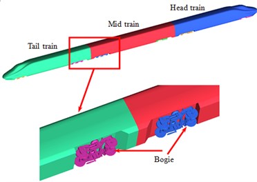
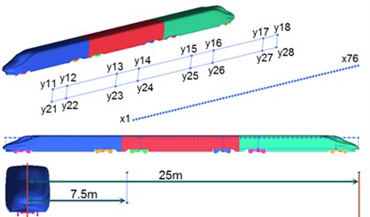
This paper took CRH2 train as the studied object and adopted 3-train formation. Each train of head train, mid train and tail train contained two bogies in the front and rear. The structure of outer windshield was adopted at train connections. The simplified model of the high-speed train was shown in Fig. 1. The dimension parameters of the high-speed train were: 75.66 m long, 3.37 m wide and 3.52 m high. The streamline of head train was 9.12 m long. The maximum cross-section area of head train was 11.83 m².

Fig. 1Geometric model of high-speed trains

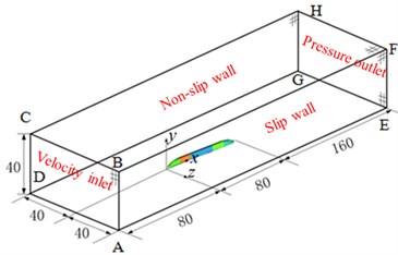
Computational domain for the aerodynamic noise of high-speed trains was shown in Fig. 2. The train length $L=$ 75.66 m was taken as the benchmark. Therefore, the computational domain was 4$L$ long, $L$ wide and 0.5$L$ high. The nose tip of head train was $L$ away from inlet. The nose tip of tail train was 2$L$ away from outlet. The train was 0.2 m away from the ground where the track was. The cross-section ABCD in front of high-speed trains was velocity inlet boundary. When the numerical computation was conducted, velocity was 350 km/h (97.222 m/s). The cross-section EFHG in the rear of high-speed trains was pressure outlet boundary. It was one standard atmospheric pressure. The cross-section BFHC above the high-speed train, CDGH at the left side of the high-speed train and ABFE at the right side of the high-speed train were set as symmetric boundary conditions. The surface of high-speed trains was set as fixed boundary which was non-slip wall boundary condition. To simulate ground effect, the ground ADGE was set as slip ground. Its slip velocity was the running speed of the train.

Fig. 2Computational domain for the aerodynamic noise of high-speed trains

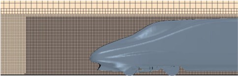
Trimmer grid was used to generate the grids of computational domain of high-speed trains. The grids of the boundary layer were divided on the surface of high-speed trains. In the meanwhile, the area of grid refinement was set around the high-speed train. The maximum size on the surface of the train was 80 mm; the maximum size of space grids was 1500 mm; the maximum size of encrypted regional grids around the train was 40 mm. To eliminate the impact of grid density on computational results, three sets of grids were divided to test the independence of grids. Computational results for three sets of grids were shown in Table 1. Drag coefficient $C_d$ and lift coefficient $C_l$ were defined as:

wherein, $F_d$ and $F_l$ were aerodynamic drag and lift borne by the high-speed train; $\rho$ referred to air density; $V$ stood for the running speed of high-speed trains; $S$ represented the maximum cross-section area of train body of high-speed trains.

As shown in Table 1, the computed drag coefficient of the second set of grids presented the change of 0.44 % compared with the first set of grids, and the lift coefficient of tail train presented the change of 3.73 %. The computed drag coefficient of the third set of grids presented the change of 0.12 % compared with the second set of grids, and the lift coefficient of tail train presented the change of 0.78 %. The change of computational results of the third set of grids was within 1 % compared with the second set of grids. Therefore, the size of the second set of grids was selected as the final grid. Finally, there were 16.48 million elements and 16.96 million nodes in the complete train, where the bogie had 50123 elements and 60923 nodes. Fig. 3 showed the schematic diagram for the grids of the complete train, head train and bogies. Local refinement was conducted around the complete train.

Fig. 3Schematic diagram for the grids of high-speed trains

a) The complete train

b) Head train

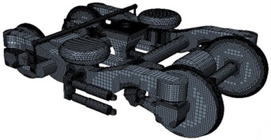
c) Bogie

4. Aerodynamic noise characteristics of high-speed trains

4.1. Distribution characteristics of flow field at bogies

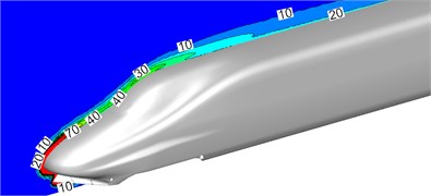
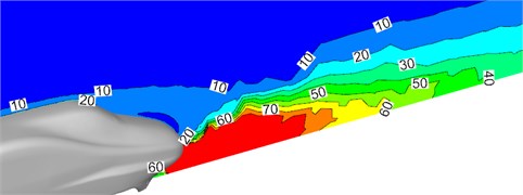
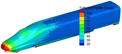
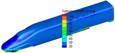
Fig. 4 showed the distribution of turbulence kinetic energy of the complete train and head train on the longitudinal central plane. Fig. 5 displayed the contour for the distribution of turbulence kinetic energy on the surface of head train. As displayed from Fig. 4, there was high turbulence kinetic energy at the nose tip of head train and in the rear of nose tip of tail train. In addition, fluid separation and reorganization occurred alternately in this area. As a result, it could be seen that head train was the main aerodynamic noise source of high-speed trains. Meanwhile, it could be seen from Fig. 5 that there was large turbulence kinetic energy in the bogie area and it was mainly at the leeward side of the bogie area. Thus, the bogie area was also the main aerodynamic noise source of high-speed trains.

Fig. 4Distribution of turbulence kinetic distribution around the high-speed train

a) The complete train

b) Head train

c) Tail train

Fig. 5Distribution of turbulence kinetic distribution of bodies of high-speed trains

b) Head train

c) Tail train

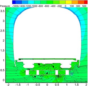
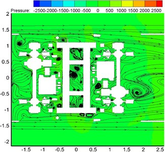
Fig. 6 showed the velocity streamline when the high-speed train ran on the ground at the speed of 350 km/h. As displayed from Fig. 6, there were many vortexes at the position of bogies. The flow velocity of airflow flowing through bogies was large. Therefore, pressure in front of bogies was more than that in the rear of bogies. In addition, vortexes appeared between disc brake device and frame support, below air spring, in front of and outside the frame. As displayed from Fig. 6(b), large vortexes were also in the rear of wheel-sets due to the blocking function of bogie skirt plates. Thus, it was clear that this position would easily lead to the accumulation of wind sand and snow under the climate condition of wind sand and snow. It was very necessary to consider the distribution of flow field in the area in the case of conducting optimization design for the streamline of bogies, reducing drag and noise, preventing the accumulation of sand and snow and the freeze of accumulated snow and so on.

Fig. 6Velocity streamline at the first bogie of head train

a) Horizontal cross-section

b) Longitudinal cross-section

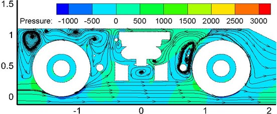
c) Vertical cross-section

4.2. Pressure at the nose tip of head train of high-speed trains

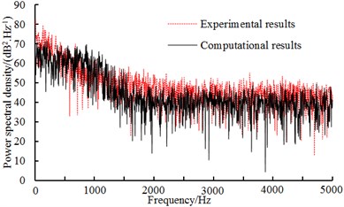
When the high-speed train ran at a certain speed, fluctuation pressures of all observation points were compared and analyzed. It could be found that fluctuation pressure at the streamline part of head train presented great changes and fluctuation pressure at the nose tip of head train reached the maximum value. It was because airflow separated when flowing through the nose tip of the train. A part of airflow flew upward along the surface of the train while a part of airflow flew downward along the bottom of the train, which resulted in the most intense airflow disturbance and separation at the nose tip of the train. Therefore, this paper took the observation point at the nose tip of head train as an example to analyze time-domain and frequency-domain characteristics of fluctuation pressure. Fig. 7 displayed the time-domain curve of fluctuation pressure at the nose tip of head train when the train ran at the speed of 350 km/h. According to the computational result in time-domain, power spectral density can be obtained and compared with the experimental result to verify the correctness of the computational model, as shown in Fig. 8.

As displayed from Fig. 7 and Fig. 8, fluctuation pressure on the surface of high-speed trains presented serious fluctuation in the time domain and changed unregularly. Fluctuation pressure was a broadband signal in the frequency domain and main energy was mainly in the low frequency. Within the frequency of 200 Hz-2000 Hz, power spectral density decreased quickly with the increased frequency. When the analyzed frequency was higher than 2000 Hz, power spectral density tended to be stable and changed little. The consistency between simulation and experiment was good, so the computational model in this paper was reliable.

Fig. 7Pressure of the observation point at the nose tip of head train

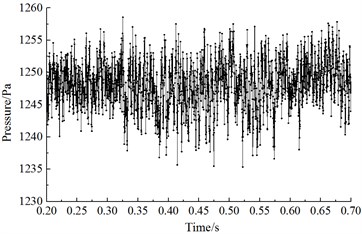
Fig. 8Comparison of PSD of the observation point at the nose tip of head train

4.3. Analysis on the aerodynamic noise of high-speed trains

4.3.1. Arrangement of noise observation points

Noises of high-speed trains along railway lines are one of noise problems of high-speed trains that people pay special attention to. Far-field noises will cause strong noise pollution along railway lines. To study the far-field aerodynamic noise characteristics of high-speed trains, 76 noise observation points were uniformly arranged along the longitudinal direction of the train ($X$-axis) in the position which was 3.5 m high from the track and 25 m away from the center line of track according to the international standard ISO3095-2005 [31]. The distance of two adjacent longitudinal observation points was 1 m. In the position which was 3.5 m high from the track and 7.5 m away from the center line of track, 8 noise observation points were arranged along the longitudinal direction of the train. One noise observation point (Serial numbers of observation points were $y11$, $y12$, $y13$, $y14$, $y15$, $y16$, $y17$ and $y18$) was arranged respectively at the nose tip of head train, the nose tip of tail train, and six bogies. In the position which was 1.2 m high from the track and 7.5 m away from the center line of track, 8 noise observation points were arranged along the longitudinal direction of the train. One noise observation point (Serial numbers of observation points were $y21$, $y22$, $y23$, $y24$, $y25$, $y26$, $y27$ and $y28$) was arranged respectively at the nose tip of head train, the nose tip of tail train, and six bogies. Fig. 9 showed the arrangement and serial numbers of observation points used to compute the aerodynamic noise of high-speed trains.

Fig. 9Distribution for the far-field observation points of aerodynamic noises

4.3.2. Aerodynamic noises which were 25 m away from the center line of track

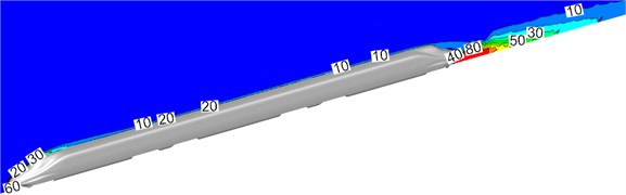
Fig. 10 showed A-weighted sound pressure levels of longitudinal observation points when the high-speed train ran at the speed of 350 km/h. Observation points were 25 m away from the center line of track and 3.5 m high from the rail surface.

As shown in Fig. 10, the distribution of sound pressure levels of longitudinal aerodynamic noise of high-speed trains presented the trend of decrease. Due to these bogies in the high speed train, sound pressure levels had some obvious peaks. The sound pressure level of noise observation points at the first bogie of head train was the largest and reached the maximum value. Total sound pressure levels reached local maximums at the second bogie of head train, the first and second bogie of mid train, and the first and second bogie of tail train. When the transition was $x=$ 6 m at the nose tip of head train, the sound pressure level of far-field noises quickly increased and increased by 5.2 dBA at most. Then, the sound pressure level of the complete train gradually decreased. When the transition was $x=$ 6 m at the nose tip of head train, the sound pressure level of far-field noises reached the maximum value among noise observation points of the complete train, namely 88.9 dBA. At the streamline part of tail train, noise sound pressure level attenuated quickly and the maximum attenuation value was 9.4 dBA. Similarly, total noise sound pressure levels reached local maximums around the first and second bogie of mid train, and the first and second bogie of tail train, which can be seen from six positions in Fig. 10.

Fig. 10Sound pressure levels of longitudinal observation points

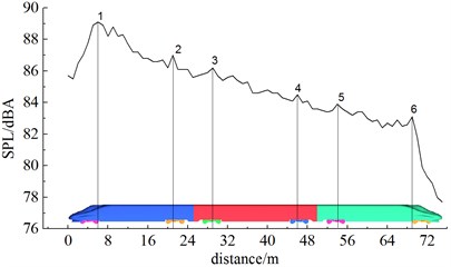
Fig. 11 showed the distribution of the A-weighted sound pressure levels of longitudinal observation points along the longitudinal direction of the train when the high-speed train ran at different speeds (250 km/h and 300 km/h). Noise observation points were 25 m away from the center line of track and 3.5 m high from the rail surface.

Fig. 11Sound pressure levels of longitudinal observation points at different running speeds

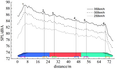
As displayed from Fig. 11, the sound pressure level of longitudinal observation points obviously increased with the increase of running speed. When the running speed was 250 km/h, 300 km/h and 350 km/h, maximum sound pressure levels were 83.4 dBA, 86.7 dBA and 88.9 dBA respectively among longitudinal observation points and increased amplitudes were 3.3 dBA and 2.2 dBA, which showed that the increased amplitude of aerodynamic noises of the same observation point was smaller with the increased speed. When running speed increased from 250 km/h to 350 km/h, the maximum sound pressure level rose by 5.5 dBA. From Fig. 11, similarly, it could be seen that total sound pressure levels reached local maximums at the first and second bogie of head train, the first and second bogie of mid train, and the first and second bogie of tail train when the high-speed train ran at different speeds.

4.3.3. Aerodynamic noises which were 7.5 m away from the center line of track

Fig. 12 displayed the distribution of A-weighted sound pressure levels of 8 noise observation points along the longitudinal direction of the train in the position which was 3.5 m high from the track and 7.5m away from the center line of track. Serial numbers of noise observation points were $y11$, $y12$, $y13$, $y14$, $y15$, $y16$, $y17$ and $y18$. As displayed from Fig. 12, A-weighted sound pressure levels were 90.0 dBA, 94.5 dBA, 89.5 dBA, 89.4 dBA, 86.3 dBA, 86.4 dBA, 85.1 dBA and 81.6 dBA respectively at the nose tip of head train, the nose tip of tail train, and six bogies. Decreased amplitudes were –4.5 dBA, 5.0 dBA, 0.1 dBA, 3.1 dBA, –0.1 dBA, 1.3 dBA and 3.5 dBA. The sound pressure level of noise observation point $y12$ around the first bogie of head train reached the maximum value.

Fig. 12Distribution for the sound pressure level of observation points

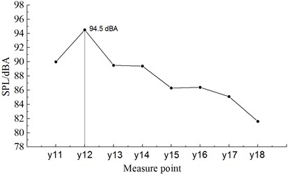
Fig. 13 displayed the distribution of A-weighted sound pressure levels of 8 noise observation points along the longitudinal direction of the train in the position which was 1.2 m high from the track and 7.5m away from the center line of track. Serial numbers of noise observation points were $y21$, $y22$, $y23$, $y24$, $y25$, $y26$, $y27$ and $y28$. As displayed from Fig. 13, A-weighted sound pressure levels were 90.5 dBA, 97.1 dBA, 91.0 dBA, 91.1 dBA, 88.4 dBA, 89.1 dBA, 88.3 dBA and 83.8dBA respectively at the nose tip of head train, the nose tip of tail train, and six bogies. Decreased amplitudes were –6.6 dBA, 6.1 dBA, –0.1 dBA, 2.7 dBA, –0.7 dBA, 0.8 dBA and 4.5 dBA. The sound pressure level of noise observation point $y22$ around the first bogie of head train reached the maximum value.

Fig. 13Distribution for the sound pressure levels of observation points

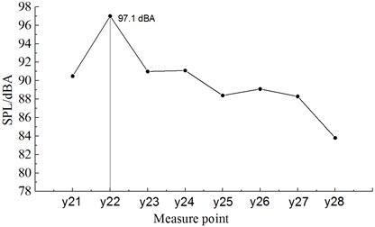
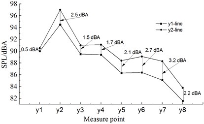
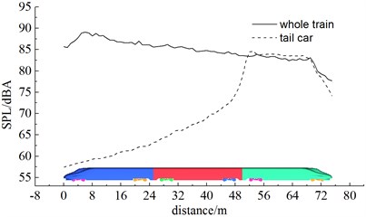
Fig. 14 showed the comparison of A-weighted sound pressure levels of 16 noise observation points along the longitudinal direction of the train in the position which was 1.2 m and 3.5 m high from the track. As displayed from Fig. 14, the sound pressure level of observation point $y1$-line was less than that of $y2$-line. Thus, it was clear that the sound pressure level was higher when noise observation points were closer to the ground. Sound pressure levels of observation point $y1$-line at the nose tip of head train, the nose tip of tail train, and six bogies were 0.5 dBA, 2.5 dBA, 1.5 dBA, 1.7 dBA, 2.1 dBA, 2.7 dBA, 3.2 dBA and 2.2 dBA higher than those of observation point $y2$-line. To sum up, it could be seen that noise observation points should be arranged at the cross-section of $y2$, namely at the first bogie of head train, when the aerodynamic noise of high-speed trains was measured.

Fig. 14Comparison for the sound pressure levels of observation points

4.3.4. Spectral characteristics of aerodynamic noises

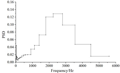
Fig. 15 displayed the distribution of one-third octave at the observation point $x6$ when the high-speed train ran at the speed of 350 km/h. Fig. 16 displayed the distribution of power spectral density at the observation point $x6$ when the high-speed train ran at the speed of 350 km/h. From the comparison of Fig. 15 and Fig. 16, the far-field aerodynamic noise of the high-speed train was a kind of broadband noise, whose main energy was within the frequency of 613 Hz to 2500 Hz.

Fig. 15Analysis of one-third octave at the observation point x6

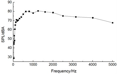
Fig. 16Distribution for the power spectral density of the observation point x6

4.4. Contribution to the aerodynamic noise of high-speed train

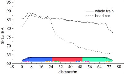
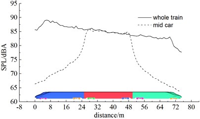
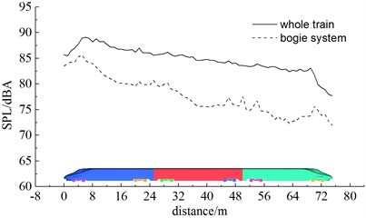
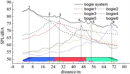
As shown in Fig. 17, the complete train, head train, mid train and bogie system (6 bogies) were noise sources and the comparison of sound pressure levels at the longitudinal plane was obtained when the high-speed train ran at the speed of 350 km/h. Fig. 18 displayed the contribution of bogie system to far-field aerodynamic noises. As displayed from Fig. 17, the contribution of various train bodies was mainly noise radiation vertical to train bodies. Head train made the greatest contribution to total noises. The maximum sound pressure level was 87.6 dBA, followed by mid train, bogie system and tail train whose maximum sound pressure levels were 86.9 dBA, 85.7 dBA and 84.6 dBA. The maximum sound pressure levels of head train, mid train, bogie system and tail train were 1.3 dBA, 2 dBA, 3.2 dBA and 4.3 dBA different from that of the complete train. From the analysis of Fig. 18, it could be seen that the contribution of bogie 1, 2, 3, 4, 5 and 6 to bogie system was mainly from noise radiation vertical to train bodies. Their maximum sound pressure levels were 85.3 dBA, 77.2 dBA, 76.9 dBA, 73.7 dBA, 74.3 dBA and 73.9 dBA respectively which were 3.6 dBA, 11.7 dBA, 12 dBA, 15.2 dBA, 14.6 dBA and 15 dBA different from that of the complete train. Thus, it was clear that the first bogie of head train made the greatest contribution to the far-field aerodynamic noise of the high-speed train and was main aerodynamic noise source. To reduce the far-field aerodynamic noise of the high-speed train, it was advised to reduce noises at the head train and the first bogie of head train. The noise reduction effect was very obvious.

Fig. 17Contribution of various components to aerodynamic noises

a) Head train

b) Mid train

c) Tail train

d) Bogie

Table 2Contribution of aerodynamic noises

Component	Maximum sound pressure level (dBA)	Difference value of sound pressure level with the complete train (dBA)
The complete train	88.9
Head train	87.6	1.3
Mid train	86.9	2.0
Tail train	84.6	4.3
Bogie system	85.7	3.2
Bogie 1	85.3	3.6
Bogie 2	77.2	11.7
Bogie 3	76.9	12.0
Bogie 4	73.7	15.2
Bogie 5	74.3	14.6
Bogie 6	73.9	15.0

Fig. 18Contribution of bogie system to aerodynamic noises

5. Conclusions

This paper adopted DES and FW-H acoustic model to conduct numerical computation for the aerodynamic noise of the high-speed train, analyzed the aerodynamic flow behavior and far-field aerodynamic noises and achieved the following conclusions:

1) The aerodynamic noise sources of the high-speed train were distributed at the nose tip and pilot of head train and bogie area of different train bodies.

2) Through the comparative analysis of total sound pressure levels of noise observation points (25 m away from the center line of track and 3.5 m away from the rail surface) of the high-speed train, the total sound pressure level of the observation point $x6$ which was 25 m away from the nose tip of head train was the largest, namely 88.9 dBA (The high-speed train ran at the speed of 350 km/h). Therefore, noise observation points should be arranged in this position in future experimental research.

3) Through computing the aerodynamic noise of the observation point which was 7.5 m away from the center line of track, the result showed that the sound pressure level of aerodynamic noises was the largest at the first bogie of head train and the sound pressure level was greater when it was closer to the ground.

4) The far-field aerodynamic noise of the high-speed train was a kind of broadband noise; whose main energy was within the frequency of 613 Hz to 2500 Hz.

5) Through computing the contribution of aerodynamic noises of the high-speed train, the result showed that the greatest contribution to the far-field aerodynamic noise of the complete train was made by head train, mid train, bogie system and tail train in order. 6 bogies made different contributions to bogie system, namely two bogies of head train, first bogie of mid train, two bogies of tail train, and second bogie of mid train. The first bogie of head train was the main aerodynamic noise source of the high-speed train. To reduce the aerodynamic noise of the high-speed train, it was advised to analyze the noise reduction mechanism of head train and bogie system. Its noise reduction effect will be very obvious.