Fault diagnosis of rolling element bearing based on wavelet kernel principle component analysis-coupled hidden Markov model

1. Introduction

HMM has been used in fault diagnosis of rotating machinery widely [1-5]. However, it could not solve the multi-channel data fusion problem. Many machine condition monitoring techniques have been proposed based on multi-channel data acquisition system [6]. The current data fusion techniques are mainly classified into three categories: data-level fusion, feature-level fusion and decision-level fusion. Vibration and current signals were fused basing on Dempster-Shafer (DS) to improve the diagnostic accuracy [7]. Some vibration parameters such as RMS, peak and peak to peak were used in the detection defects in the bearing [8]. In order to obtain better diagnostic result, the waterfall fusion model was adopted by fusing information from two different kinds of sensors: the accelerometer and load cell [9]. CHMH [10] was first proposed as a novel sensory fusion architecture to solve the data fusion problem in audio-visual speech recognition (AVSR). Xie [11] proposed a coupled hidden Markov model approach to video-realistic speech animation and realistic facial animations driven by speaker independent continuous speech was realized. In paper [12] the dependent faults occurring over time were diagnosed successfully by the proposed coupled factorial hidden Markov model method. In paper [13] the spatial and temporal dynamics in multi-channel electrocorticographic (ECoG) time series was investigated using CHMM. Though CHMM has been used widely in the above stated aspects, very few papers presented its using in fault diagnosis of rolling element bearing. The CHMM was used in rolling element bearing fault diagnosis and performance degradation assessment respectively in paper [14] and paper [15], and satisfactory experiment analysis results were obtained. So the using of CHMM in fault diagnosis of rolling element bearing is studied and the WKPCA is used as feature extraction method in the paper.

2. Wavelet kernel principle component analysis

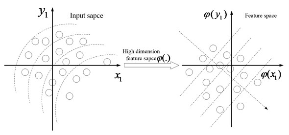
Various feature parameters are expected to be obtained so as to reflect the running state of the machinery comprehensively. However, the efficiency of the subsequent intelligent diagnosis will be decreased greatly when too many feature vectors are used as the input vectors. Besides, some of the feature parameters are redundant and useless which will decrease the accuracy of intelligent diagnosis to some extent. Principle components analysis (PCA) and the improved PCA method-kernel principle component analysis (KPCA) [16, 17] are the common used linear and non-linear feature dimensionality reduction methods to solve the above contradiction. The schematic diagrams of PCA and KPCA can be referred to Fig. 1 and Fig. 2. KPCA not only owns the virtues of PCA, but also can analyze the non-linear problems which PCA could not. Besides, the KPCA has other advantages which can be referred to the paper [18]. Though KPCA improve the PCA greatly, there are still some defects in the traditional KPCA: firstly, the selection of kernel function in the traditional KPCA is based on experience. Secondly, there is not criterion for selection of the relative parameters of kernel function. Any functions can be fitted by the wavelet function [19] in theory, so in the paper a novel features reduction method named WKPCA is proposed: the wavelet function is used as the kernel function instead of the common used radial basis function (RBF) in KPCA, and the wavelet function can increase the non-linear mapping ability of KPCA greatly. The relative definitions and theory of WKPCA are given as the following.

Fig. 1The schematic diagram of PCA

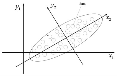
Fig. 2The schematic diagram of KPCA

Definition 1 [20]: Kernel is a function $K$ which satisfies the following equation for any $x(x\in R^n)$:

where $x^{\text{'}}$ represents the transpose and $\varphi (.)$ represents a mapping from the data space $R^n$ to the feature space $F$, and the relationship of them can be shown as following:

It not only can calculate the inner product more efficiently but also need not calculate mapping $\varphi$ process explicitly. The kernel function must satisfy the requirement of Mercer [21].

Theorem 1 [22]: Supposing $K$ is a continuous symmetric function $K\in L_{\infty }(R^n\times R^n)$ which makes the integral operator $T_K:L_2\left(R^n\right)\to L_2\left(R^n\right)$:

to be positive. That is to say the following relationship can be obtained:

In Eq. (4), the $\otimes$ symbol represents convolution algorithm. $K\left(x,x^{\text{'}}\right)$ could be used as the representation of dot product in the feature space if the above conditions can be satisfied.

The kernel function $K(x,x^{\text{'}})=K(x-x^{\text{'}})$ satisfies the requirement of Mercer which is given in theorem 2.

Theorem 2 [23]: If the translation invariant kernel function $K(x,x^{\text{'}})=K(x-x^{\text{'}})$ is an allowable kernel whose fourier transform (FT) must satisfy the following condition:

Wavelet function has the peculiar characteristics of multi-resolution analysis compared with the common used kernel functions such as RBF used in the traditional KPCA. The wavelet function can fit any function much more precisely, so the wavelet function is combined with PCA instead of the common used kernel function such as RBF, so much stronger non-linear mapping capability can be obtained. The combination of wavelet function with PCA is named wavelet kernel principal component analysis also called WKPCA for short.

Supposing $\psi \left(x\right)\in L_2\left(R\right)$ is a mother wavelet function, $x$, $x\in R^n$, and a translation invariant wavelet kernel function satisfying the requirement of Mercer can be constructed as following [22]:

where $a_i$ is the scale factor.

The requirement of Mercer is not only satisfied but also the properties of the wavelet function are considered when the wavelet kernel function is being constructed. The wavelet construction kernel function meeting the wavelet framework conditions has obvious advantage because it takes into account the sparseness of the training data and the complexity of the constructed kernel functions. Mexican hat wavelet function is a kernel function meeting the wavelet framework conditions [24]. The Mexican hat wavelet function shown in Eq. (7) is used to construct the translation invariant kernel function:

The constructed translation invariant wavelet kernel function is shown in Eq. (8):

The proof of Mexican hat wavelet satisfying Theorem 2 is given as following.

With regard to the Mexican hat wavelet shown in Eq. (9):

In Eq. (9), $\gamma$ is the scale factor same as the meaning of ${\alpha }_i$ shown in Eqs. (6) and (8). The Eq. (10) can be obtained:

From the above, the proof of Mexican hat wavelet satisfying Theorem 2 is obtained which can be used to construct the allowable kernel function.

3. CHMM

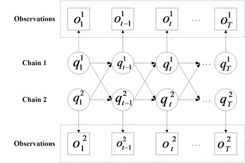
CHMM is constituted by multi-HMM chains which couple through cross-time and cross-chain conditional probabilities as illustrated in Fig. 3 and Fig. 4, and the CHMM can be regarded as a special case of dynamic Bayesian network. The observations of each chain in CHMM are decided by the corresponding state in the same chain. Besides, the unobservable state sequence can be only estimated by the observation sequence. The above two characteristics of CHMM are similar to HMM. Different from HMM, all the state variables in different chains may be contained at certain time slice in the states of the CHMM system. The states of all chains in the previous time slice decide the state in each chain. So much comprehensive fault diagnosis result of bearing can be obtained using CHMM because it has a potential to fuse data from multi-channel. The following is the basic theory introduction of a two-chain CHMM.

Fig. 3The schematic of HMM

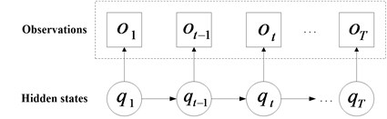
Fig. 4The schematic diagram of CHMM

4. Experiment

The flow chart of the proposed method based on WKPCA-CHMM is shown in Fig. 5 and the specific details of each step are given as following:

Step 1: Data collection: collect the signals of the four states (normal state, outer race fault state, rolling element fault state and inner race fault state) of rolling element bearing using double channel accelerator sensors.

Step 2: Data separation and feature extraction: separate the data of the eight channel signals into 50 groups (The 1-40th groups are used as CHMM training data and 41th-50th groups are used as testing data) respectively and 400 groups are obtained in all. There are 1024 points in each group. Apply the eleven time-domain statistical indexes (The 11 indexes and their corresponding calculation formulas are shown in Table 1) and one time-frequency domain index (the wavelet packet energy entropy (WE) which will be stated in the following chapter) to each group data.

Noting: The 11 indexes are the traditional common used time-domain statistical feature vectors and they can reflect the running state correctly when the fault signal is linear. The signals usually take on non-linear characteristic when fault occurs in machinery, so the time-frequency index is also need so as to capture the characteristic of the fault signal. In the paper, the wavelet packet energy entropy (WE) is used as time-frequency index which will be discussed in the Subsequent chapters.

Step 3: Dimensionality reduction: apply WKPCA to the feature vectors obtained in step 2 in order to obtain dimensionality reduction feature vectors.

Step 4: CHMM models training: use the dimensionality reduction training feature vectors to train four CHMM models (normal state CHMM, inner race fault state CHMM, outer race fault state CHMM and rolling element fault state CHMM).

Step 5: Diagnosis: input the dimensionality reduction testing feature vectors into the trained four state CHMMs in step 4 and fault diagnosis results are obtained.

Fig. 5The framework of the proposed method

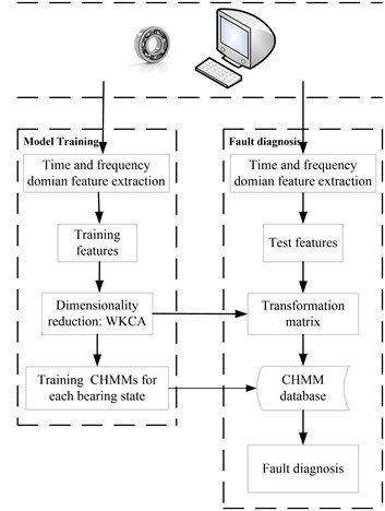
Fig. 6The test rig

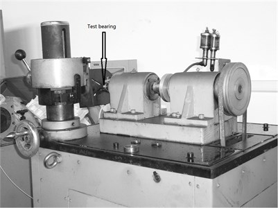
The test rig is shown in Fig. 6. The two ends of the shaft are supported by two rolling element bearings, and the right end is detachable which is convenient for replacement of the test rolling element bearings. The shaft is driven by AC motor and connected by coupling. The rated power of the AC is 1.1 kW. The test rig is equipped with hydraulic position and clamping device which are used in fixing the outer race of rolling bearing. The inner race, rolling element and outer race of the test rolling bearings are eroded with very tiny point corrosions respectively using Electrical Discharge Machining (EDM) technology to simulate the three kinds of faults of the rolling bearing. The type of the test rolling bearing is GB203. The outer race is fixed on the bench and the inner race rotates synchronously with the shaft in the test process. The rotation frequency of the shaft is $f_r=$12 Hz. The parameters and the rotation frequency of the test rolling element bearings are shown in Table 2.

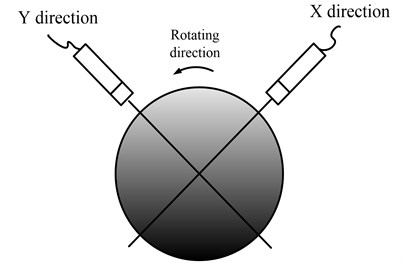
One sensor is installed in the traditional vibration data collection method. In the paper the two accelerometers are installed in the same one bearing case synchronously, and the two installed directions are shown in Fig. 7.

Fig. 7The installation direction of the two sensors

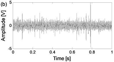
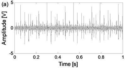
The four states of the test rolling bearings are carried on respectively and the corresponding time-domain waveforms of the two channel signals from the same data collection point of the four states are shown in Fig. 8. The sampling frequency is $f_s=$25.6 kHz.

It is usually taking on non-gaussian and non-linear characteristic whatever the condition of the rolling bearings is (normal or fault). The time-frequency analysis method is a very effective non-linear and non-gaussian signal handling tool to extract the non-linear features buried in the original signal. In the paper, the wavelet packet energy entropy is used as the time-frequency indicator whose calculation process is shown as following:

Apply the wavelet packet transform (WPT) to the original signal and the energies $E_i(i=2^N$, $N$ is the decomposition level) named wavelet packet energy on each node is obtained which is the division of the original signal in the time-frequency domain. In theory, much better frequency-domain performance could be obtained with the bigger value of $N$. However, the amount of calculation will also be increased with the bigger value of $N$. So, the value of $N$ is selected 3 as compromising here, and the satisfactory frequency-domain performance could be obtained with the following verification of experimental results. The wavelet packet energy entropy (WE) is defined as in Eq. (15):

In Eq. (15), $p_i$ represents probability distribution. The Normalized wavelet packet energy and wavelet packet energy entropy results of the signals shown in Fig. 8 are summarized in Fig. 9.

Fig. 8The time-domain waveforms of the two channels signals from the same data collection point of the four states

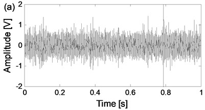
a) The time-domain waveform of channel 1 of normal state

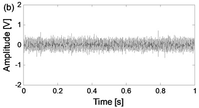
b) The time-domain waveform of channel 2 of normal state

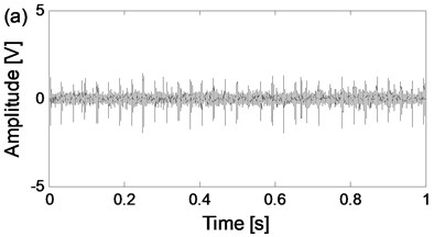
c) The time-domain waveform of channel 1 of outer race fault state

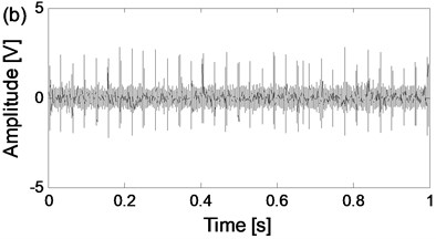
d) The time-domain waveform of channel 2 of outer race fault state

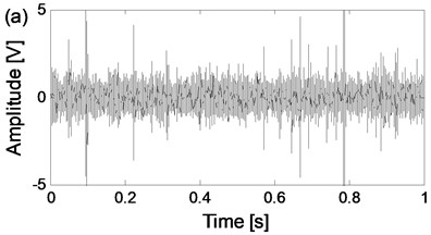
e) The time-domain waveform of channel 1 of rolling element fault state

f) The time-domain waveform of channel 2 of rolling element fault state

g) The time-domain waveform of channel 1 of inner race fault state

h) The time-domain waveform of channel 2 of inner race fault state

So, the dimensionality of training feature vectors of every channel is 4×50×12. Apply WKPCA to the 4×40×12 feature vectors of channel 1 and 2 respectively and the analysis results are shown in Fig. 10 and Fig. 11. In Fig. 12, the curves of classification result with the number of kernel principle components (PC) is given, and it is evident that the correction ratio would be almost unchanged when the number of PC varies from 3-12. Though in theory the correction ration will obtain the biggest value when the number of PC is selected 12 as shown in Fig. 12, the classification speed will be decreased too much. So, the number is selected 3 as compromising to ensure the classification speed, and the classification correction is guaranteed at the same time. From the dimensionality reduction result it is evident that the dimensionality of the feature vectors is reduced to 4×40×3 respectively.

Fig. 9Normalized wavelet packet energy and wavelet packet energy entropy

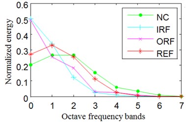
a) The normalized energy of channel 1

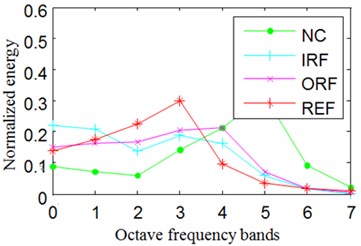
b) The normalized energy of channel 2

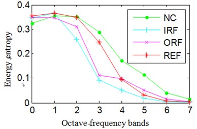
c) The energy entropy of channel 1

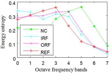
d) The energy entropy of channel 2

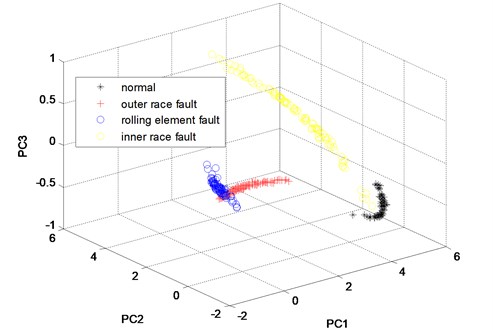
Fig. 10The three principle components of the twelve features of the channel 1 of the four states analyzed by WKPCA method

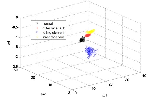
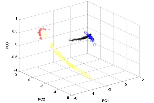
From Fig. 10, it can be seen that, almost all of the four states’ sample vectors (* represents the sample vectors of normal state, + represents the samples vectors of outer race fault state, blue o represents the sample vectors of rolling element fault state and yellow o represents the sample vectors of inner race fault state) are classified correctly. Though small amount of sample vectors of outer race fault state and inner race fault state are misclassified in Fig. 11, most of the other sample vectors of the four states are classified correctly. In order to verify the advantage of WKPCA over KPCA, the analysis result of the signals shown in Fig. 8 using KPCA are given in Fig. 13 and Fig. 14. The advantages of WKPCA over KPCA is obvious compared the Fig. 10 and Fig. 11 with Fig. 13 and Fig.14: Much more amount of sample vectors of the four states are misclassified compared Fig. 13 and Fig. 14 with Fig. 10 and Fig. 11. Besides, the better clustering result which has bigger classes distance and smaller intra-class distance is evident in Fig. 10 and Fig. 11 compared with the results obtained in Fig. 13 and Fig. 14.

Fig. 11The three principle components of the twelve features of the channel 2 of the four states analyzed by WKPCA method

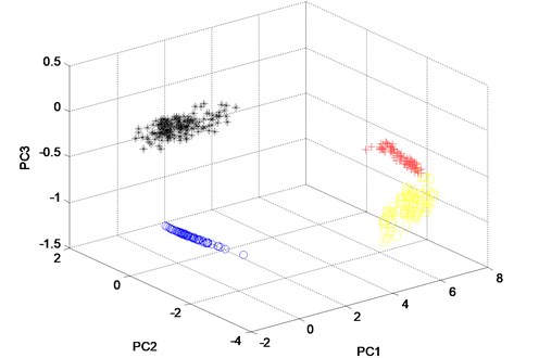
Fig. 12The curves of classification result with the number of kernel principle components

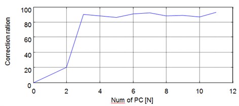
Fig. 13The three principle components of the twelve features of the channel 1 of the four states analyzed by KPCA method

Use the 4×40×3×2 feature vectors as training feature vectors respectively and the normal state CHMM, outer race fault state CMHH, rolling element fault state CHMM and inner race fault state CHMM diagnosis trained models are erected respectively. Then input the 4×40×3×2 feature vectors as testing feature vectors into the above four trained diagnosis models, and the diagnosis results are obtained and shown in Fig. 15(c) at last. From the Fig. 15(c) the ten groups of the testing feature vectors of the four states are classified corrected completely.

Fig. 14The three principle components of the twelve features of the channel 2 of the four states analyzed by KPCA method

In order to verify the advantage of CHMM over HMM, the diagnosis result based on WKPCA-HMM of the two channel signals of the four states are also carried out respectively. Same as the above CHMM models training and testing process: firstly, use the 4×40×3×2 as training feature vectors respectively and the normal state HMM, outer race fault state MHH, rolling element fault state HMM and inner race fault state HMM diagnosis trained models of the two channel signals are erected respectively, then input the 4×10×3×2 feature vectors as testing feature vectors into the above eight trained diagnosis models, and the diagnosis results are obtained and shown in Fig. 15(a) and Fig. 15(b) respectively. Compared Fig. 15(a) and Fig. 15(b) with Fig. 15(c), the advantages of the proposed method are obvious: in Fig. 15(a) the are three groups of rolling element fault state testing feature vectors are misclassified as normal state. In Fig. 15(b) there is not only one group of rolling element fault state testing feature vector is misclassified as normal state but also there are three groups of outer race fault state testing feature vectors are misclassified as inner race fault state. Based on the above shown results, the advantage of CHMM over HMM in fault diagnosis of rolling element bearing is verified: the CHMM can fuse the information of two channels signals from the same data collection point efficiently and might also resolve the possible coupling phenomenon occurring between the two channel signals synchronously so much more reliable diagnosis result could be obtained compared with the HMM method. Besides, the dimension redundancy and dimension insufficient contraction is not only resolved but also the diagnosis efficiency and correction ratio are also increased because the WKPCA method is used as feature dimensionality method.

Besides, the computation time and correction ratio of the other three relative methods (WKPCA-HMM, RKPCA-CHMM and CHMM without dimensionality reduced) and the proposed method (WKPCA-CHMM) are shown in Table 3. Based on Table 3 the advantages of the proposed are further verified.

Fig. 15The diagnosis results based on WKPCA-HMM and WPCA-CHMM

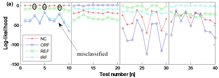
a) The diagnosis results of channel 1 signals of the four states based on WKPCA-HMM

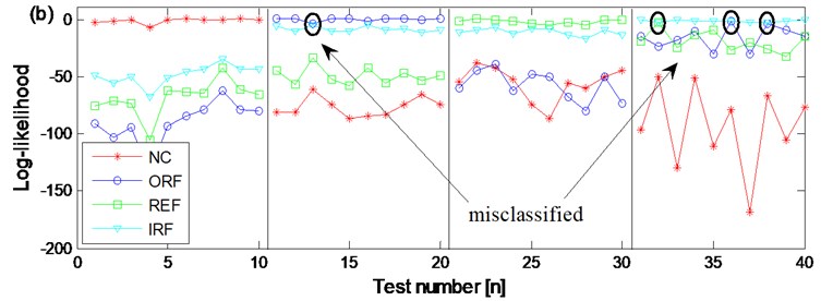
b) The diagnosis results of channel 2 signals of the four states based on WKPCA-HMM

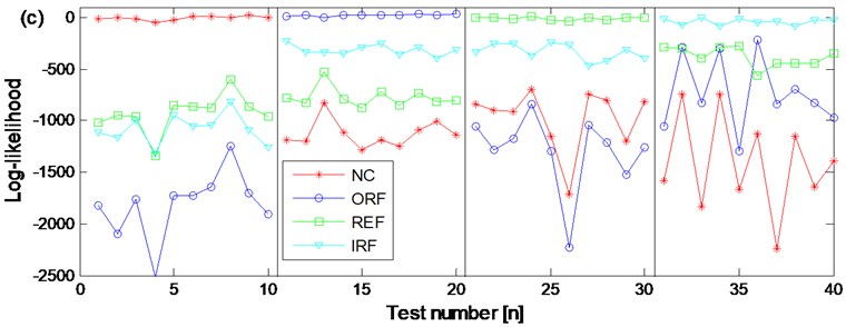
c) The diagnosis results of the two channels signals of the four states based on WKPCA-CHMM

5. Conclusions

The paper presents an integrated WKPCA-CHMM method to realize the intelligent fault diagnosis of rolling element bearing. The advantage of CHMM over HMM is following: the CHMM can fuse the information of two channel signals from the same data collection point efficiently and might also solve the possible coupling phenomenon occurring between the two channel signals synchronously. The WKPCA is used as feature dimensionality reduction method for it is not only can solve the dimension redundancy and dimension insufficient contraction but also is much more flexible than RKPCA. The feasibility and validity of the proposed method is verified through experiment. Besides, the advantages of the proposed method over other relative methods are also verified and presented.