A 2D-3D non-contact anthropometric method for daily dressing state-takes young Asian women as example

1. Introduction

As an important branch of clothing ergonomics, anthropometry is the groundwork ensuring clothing design and manufacturing. In contrast to the traditional contact measuring mode, non-contact ones can offer accurate and full-scale measured data to meet the demands of modern garment digital trend well. 3D scanning and 2D-3D conversion are the main measuring and calculating methods used in the field of non-contact anthropometry, especially the former is well-developed over the past two decades.

For 3D scanning, using laser is popular. Some researchers did related works. For example, Watanabe et al. [1] adopted a laser displacement meter to measure waist circumference and developed the new system for the non-contact measurement of abdominal cross section. Shang et al. [2] used artificial and three-dimensional laser measurement method, through which the sample data were collected in the same situation, to study the national and professional standard size measurement system. In the design of data standards, using statistical methods to analyze the data, and a comprehensive evaluation from two aspects of stability of instrument and data correlation. The practical application was taken as an example to study the tolerance range of standard data. The research works of Wang and Jiang [3] were based on the measurement principle of structured light, a laser rotating body scanning of non-contact measurement system. They gave the requiring of Made to Measure apparel production mode according to individual types and made calibration about body measurement and production in a line. Besides using laser, other researches about the method and application of 3D measuring also carried forward the non-contact measuring technique. Such as Zhang et al. [4] developed non-contact measurement of revolving body straightness method. They inspected a 1200 mm long rotating body with a spatial straightness error of a diameter of 160 mm in the 3D machine vision metrology. Pan et. al. [5] used C# and SQL database to design and implement for non contact 3D human body measurement in the human body database management system. Wang et. al. [6] proposed a non-contact 3D body data acquisition method for garment fit evaluation the distribution characteristics of the remaining space between the 3D scanning and clothing. The researches [7-10] used 3D non-contact measurement method to analyze body shape. Remondino [11] explored the generation of 3D models from uncalibrated image sequences. The study process also included the extraction of correspondences on the body using a least squares matching algorithm and the reconstruction of the 3D body model in point cloud form.

Some researches focused on 2D and 2D-3D non-contact measurement, such as Pirre and Shi [12] developed 2D image measurement system, which could determine the size of clothing. They found image-based systems were capable of providing anthropometric measurements, both in terms of accuracy and repeatability, which were better than traditional measurement methods. Yu et al. [13] adopted a wide coverage of optical design. This system could obtain high resolution images in a short distance, and through the computer program into a 3D human body model. Gu et al. [14] developed automatic pattern generation system of men’s pants, which is based on two dimensional non-contact human body measurement systems. Guo et al. [15] explored the application of the automatic clipping method in the 2Dimensional non-contact measuring system.

As for the dynamic measurement and application researches, non contact technology of human daily life activity detection include: Kurita [16, 17] developed a method for measurement of human motion, which was the electrostatic induction current non-contact type for walking motion detection. Umeda [18] developed of non-contact detection technology, which has been used to measure human vital signs. Deepak et al. [19] and Yutaka et al. [20] utilized 3D non-contact measurement method to discuss knee motion of human body. Kurita [21] developed an effective non-contact technique for the measurement of human stepping. Nicola [22] took advantage of cameras to measure and track moving surfaces of human body parts from multi-image video sequences acquired simultaneously. Yang et al. [23] adopted high speed camera to analyze the landing from different heights, the current research tries to figure out the landing vibration responses to different segments, including the lumbar, knee, hip, neck and the reacting force from ground.

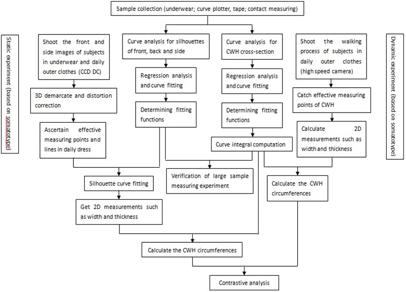
Although the previous works improved the non-contact measuring technique gradually, two of the most common problems or challenges still exist: one is the limitation on the dress of subjects, the other is the static measuring mode. That is, relatively accurate measurements of human body parts can be obtained only when subjects still stand, wearing underwear or straitjacket. In view of garment size designation of the industry, this paper introduces a 2D-3D conversion approach to generate the CWH measurements in natural daily dressing state, no matter the measuring mode is dynamic or static. Experiments prove that this method, which is free from the dressing constrains and break the static mode, can meet the accuracy requirement. In our approach, through large sample measuring experiment showed in Section 2, laws of the relative curves, such as the silhouette curves of front, back, body side and the cross-section curves of chest, waist, hip of human body, were studied in Section 3, in which their suitable fitting functions and the integral formula of the typical CWH curves were ascertained. Next, in Section 4, on the premise of somatotype, in daily dressing state, static and dynamic experiments were carried to extract the effective feature points’ information. Then 2D measurements such as the width and the thickness were measured or calculated out. With the 2D-3D conversional formulas aforementioned, the CWH measurements would be calculated finally. These numerical results and analysis are presented and discussed in Section 5. Conclusion is given in Section 6. The research route is shown in Fig. 1.

Fig. 1Research route

2. Large sample anthropological measuring experiment

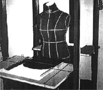
In order to ensure analysis credibility for the curves of silhouette and CWH cross-section, and the relative property between calculating measurements and actual measurements, it is necessary to build a large sample measurement database via traditional contact measuring experiment. In this paper, take Asian young women as research subjects, whose basic requirements are shown in Table 1. The sample size is 81 persons, who are random selected, determined by the known sample data of the earlier study, combining the confidence interval 95 % and the actual experimental condition. The accuracy of CWH measurements is 2 cm, according to the standard of garment size designation. Tape measure, ruler, height measure and curve plotter (Fig. 2) are the main measuring tools. Stature, Chest, Waist, Hip, heights of CWH, widths and depths of CWH, BP to BP, HP to HP, distances of C-W and W-H, Shoulder are the measuring parts, whose measuring methods refer to GB16160-2008-T. In addition, the cross section curves of CWH and the silhouette curves of front, back, and side of the 81 subjects are plotted by the curve plotter one by one. As the comparison of the later calculating measurements, measuring all the circumferences of CWH curves manually, the specific results are shown in Table 3.

3. Relative curves analysis

Curves associated with the CWH measuring and calculating include the CWH cross-section curves and the silhouette curves of the front, back and side. It is not advisable to take any one sample’s curves as the analysis basis. Therefore, the typical representative curve figures are selected. Take the chest cross-section curve as example. Firstly, divide 81 samples into three types: 0.69-0.77, 0.78-0.83 and 0.84-0.95, according to the different radius ratios of chest width/depth. Secondly, make smoothing and symmetrical process to the original figures of curves in the same radius ratio range, then overlay them and determine the mean points. Lastly, choose the curve of moderate ratio as the representative chest cross-section curve.

Fig. 2Curve plotter

3.1. CWH cross-section curves

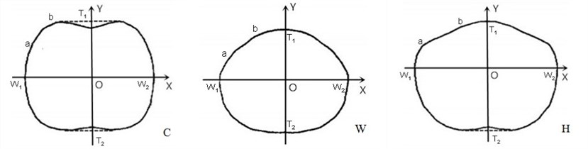
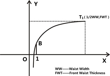
The typical CWH cross-section curves are shown in Fig. 3. For the convenience of analysis and formulation, plane-coordinate system $XOY$ is set up. For instance, the chest cross-section curve, as shown in Fig. 4, curve above $X$-axis is the front chest curve, below is the back chest curve, segment $W_1{W}_2$ is the chest width, $T_1{T}_2$ is the chest thickness, $O{T}_1$ is the front chest thickness, $O{T}_2$ is the back one. $O{W}_1=O{W}_2=$ 1/2 chest width, due to the symmetry of human body. Observe the trend of each segment curve, take the segment in ($–W_1$, 0) as example, a and b are the demarcation points, for arc $W_{1}a$, the tangent slope is larger, the curvature is less; for arc ab, the tangent slope is decreasing, the curvature is increasing; for arc $b{T}_1$, the tangent slope is minimum, the curvature is less.

Fig. 3The typical CWH cross-section curves

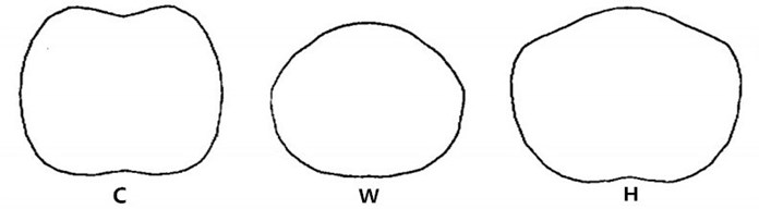
Fig. 4The typical CWH cross-section curves with XOY

3.1.1. Regression analysis

Before curve fitting and integrating, getting the thickness proportion of the front and back CWH curves is the premise. After measuring all the CWH curves obtained in the large sample experiment one by one, the regression formulas is acquired as Eq. (1). It should be noted that there are no difference of the width and thickness measurements after segmenting the CWH curves between using Eq. (1) and human judgment. Therefore, although the fitting confidences $R^2$ of the scatter plots are 0.43, 0.64, 0.51 respectively, there are no obvious significance to the final calculating results through experimental verification:

1

$\left\{\begin{array}{l}FCT=CT\times \left(1-0.5132\right),\\ BCT=CT\times 0.5132,\\ FWT=WT-\left(WT\times 0.3483+2.3891\right),\\ BWT=WT\times 0.3483+2.3891,\\ FHT=HT\times \left(1-0.6228\right),\\ BHT=HT\times 0.6228,\end{array}\right.$

where $F$ is front, $B$ is back, $T$ is thickness, $C$ is chest and $W$ is waist.

3.1.2. Curve fitting

The existing typical methods of 2D-3D conversion for circumference measurements include super-elliptic curve fitting, EE parametric spline curve fitting, binary linear regression, and quadratic regression. It is found that the first two methods need a mass of statistic data and measuring points, and errors of the last two are larger, which cannot reach the accuracy requirement of this research. According to the principles of fewer measuring points, faster calculating, and higher precision, the logarithmic, trinomial, power, binomial curves are taken as the alternative fitting curves in this paper. Take the front waist curve as example, on which extract feature points evenly, make scatter diagrams of the aforementioned curve fitting, in that order, $R^2$ are 0.9884, 0.9865, 0.9281, 0.9052. After comparing and analyzing the situation of the extracted points and fitting curves, the study found that, for the front and back segments of the CWH cross-section curve, the confidence of the logarithmic curve fitting is the best, whose shape has the similar trend with the original. Thus, the logarithmic curve is confirmed as the fitting function finally.

Take the 1/2 front waist curve (Fig. 5) as case study, its logarithmic curve equation is given as Eq. (2):

2

$Y=A\mathrm{*}\mathrm{L}\mathrm{n}\left(x\right)+B,$

where $A$ is coefficient, $B$ is intercept.

Fig. 5The abridged general view of 1/2 front waist curve

3.1.3. Intercept B

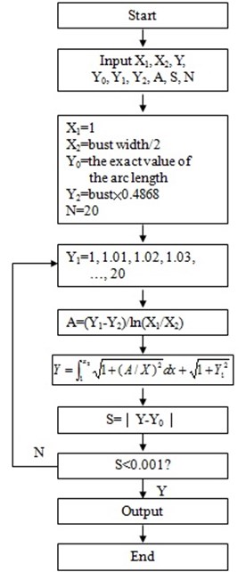
The discussion about the accurate intercept $B$ is given below. Undoubtedly, the logarithmic fitting curve determined by extracting the feature points precisely has the higher fitting precision. Measure the $CWH$ circumferences of 81 samples, calculate the integral computation of their circumferences through changing the intercept B using the successive approximation approach. Make them equal to the known measured circumference, and confirm the intercept $B$, which is regarded as the precise one. The calculation procedure is presented in Fig. 6.

Fig. 6The calculation procedure of intercept B

As for the intercept $B$ obtained using regression analysis, the relative work is described as follows. Through experiment and analysis, infer some kind of corresponding relation among the $CWH$ widths, thickness and the intercept $B$. According to the expression of correlation coefficient (Eq. (3)), the correlation coefficients of the intercept $B$ and the widths, thickness are worked out.

In accordance with the correlation, the $CWH$ intercepts are fitted by multivariable linear regression. To make the data more accurate, the correlation test among the distance of $C$-$W$, the distance of $W$-$H$ and the height, and the integral computation using different regression formulas are also conducted. After comparing errors of the integral results, Eq. (4) is written into integral program as this experimental result.

As for the intercept $B$ obtained using regression analysis, the relative work is described as follows. Through experiment and analysis, infer some kind of corresponding relation among the $CWH$ widths, thickness and the intercept $B$. according to the expression of correlation coefficient (Eq. (3)), the correlation coefficients of the intercept $B$ and the widths, thickness are worked out.

In accordance with the correlation, the $CWH$ intercepts are fitted by multivariable linear regression. To make the data more accurate, the correlation test among the distance of $C$-$W$, the distance of $W$-$H$ and the height, and the integral computation using different regression formulas are also conducted. After comparing errors of the integral results, Eq. (4) is written into integral program as this experimental result:

3

${\rho }_{XY}=\frac{Cov(X,Y)}{\sqrt{D\left(X\right)}\sqrt{D\left(Y\right)}},$

where $Cov(X,Y)$ is co-variation of $X$ and $Y$, $D\left(X\right)$, $D\left(Y\right)$ are variances of $X$ and $Y$.

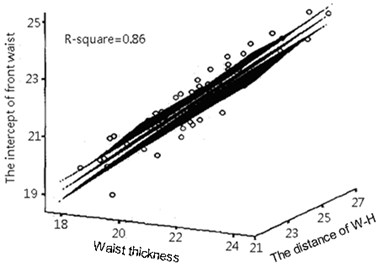
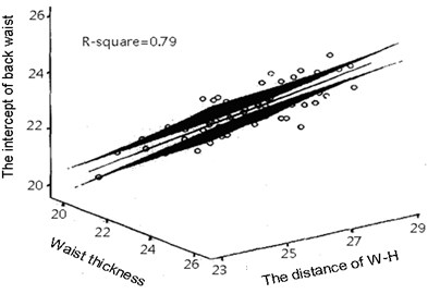
Fig. 7The scatter diagrams and responsive plane of the intercepts of the front and back waist

a)

b)

In Fig. 7:

4

$\left\{\begin{array}{l}\text{The Intercept of}FW=0.82+0.11\times WT+0.05\times \text{the distence of}W-H,\\ \text{The Intercept of}BW=1.44+0.25\times WT-0.06\times \text{the distence of}W-H,\\ \text{The Intercept of}FC=5.06-0.31\times CW+0.47\times CT,\\ \text{The Intercept of}BC=7.93-0.20\times CW+0.22\times CT,\\ \text{The Intercept of}FH=0.145+0.056\times HW+0.039\times HT+0.056\times \text{the distence of}W-H,\\ \text{The Intercept of}BH=4.315-0.235\times HW+0.397\times HT+0.115\times \text{the distence of}W-H,\end{array}\right.$

where $H$ is hip.

Take the intercepts of the front and back waist as instance, Fig. 7 shows its scatter diagrams and responsive plane.

3.1.4. Circumference calculation of the fitted curves

On the basis of Eq. (2), the girth of the fitted curve is expressed as Eq. (5). The effective integral range is (1, 1/2 width), let $k=$1/2 width, that is Eq. (6). The curvature of the curve in the range of (0, 1) is very small, and it cannot be extracted enough information and fitted in MATLAB, as a result, this paper employs the calculation method of hypotenuse (Eq. (7)) to obtain its approximate length. Through a large number of experimental verification, the error of this algorithm is minor:

5

$y=\int \sqrt{1+(a/x{)}^2}dx,$

6

$y={\int }_1^k\sqrt{1+(a/x{)}^2}dx,$

7

$a\widehat{c}\approx \sqrt{a{c^{\text{'}}}^2+c{c^{\text{'}}}^2}.$

3.2. Silhouette curves

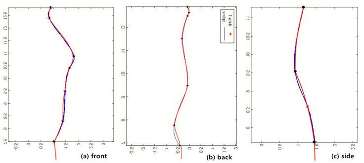
The analysis process and methods of this section is similar to the CWH cross-section curves presented in section 3.1. Here not repeat them because of the limited space. By research, the fitting functions of the silhouette curves of the front, back and side respectively are cscvn(), Spline Interplant and cscvn(). Fig. 8 shows their fitting comparison, in which the red is the typical body silhouette curves, and the blue is the fitted curves.

Fig. 8Fitting comparison

4. Static and dynamic experiment in daily dressing state

The basic information of subjects in these two experiments is as follows:

– age: 18-26;

– somatotype: thin, intermediate, plump;

– dressing types: blouse + trousers (jeans) of spring and autumn, T-shirt + tailored skirt (A-line skirt) of summer; sweater + jeans (pants) of winter.

Among them, the somatotype base is the body linear density index TNF, whose calculation is shown as Eq. (8). Table 2 shows the classification criterion. The reason why choose TNF is that TNF reflect the figure type feature of the Asian young people more better than the other universal methods such as girth difference, Rorel index, Verveck index and Bust/Height. In the base of somatotype and research of the previous large sample experiment, only three typical figure subjects are selected for case study in this section. The detailed steps are described as below:

where $W$ is weight (kg); $L$ is height (cm).

4.1. Static experiment

Main equipment: three dimensional calibration frame, fixed tripod, OLYMPUS C2500L digital camera, image capture card and a computer.

Indoor environment: room temperature 26 °C; ordinary fluorescent light.

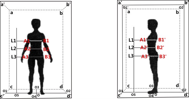
Experimental procedures: 1) Shoot the frontal and side digital images of each subject in sequence. In which, when shoot the front, the subject is required to do up hair, stand on the mark in the calibration frame, place feet shoulder width apart, raise arms whose angle with the body side is about 40°. Unlike the above, when shoot the side, the subject stand on the other mark, and her arms cling to the body without occluding the silhouette curves of the front and back. 2) Three dimensional calibration and distortion correction, to effectively reduce the measuring error caused by optical imaging. 3) Measure the related heights, lengths, and CWH widths and thicknesses. Fig. 9 shows the experimental diagrammatic sketch.

Fig. 9The static experiment arrangement

4.2. Dynamic experiment

Main hardware and software: 3D real-time motion analysis system, Raptor-E infrared high-speed camera, witch balls whose diameters are 1 cm, Cortex 3.0, and computer. Indoor environment is the same.

Fig. 10The dynamic experiment arrangement

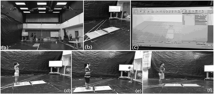
Experimental procedures: 1) Bind elastic bands and paste witch balls on the BWH locations of the subjects in natural wearing state. 2) Test the range of capturing motion and debug the system. 3) Ask the subject walk as usual in the tested space. 4) The dynamic data of the witch balls are generated in the software system Cortex 3.0.

The experimental arrangement and scene are shown in Fig. 10(a) shows the site arrangement; (b) shows the walking area; (c) shows the system which reflects the dynamic situation of the featured points; (d), (e) and (f) show the subjects of three different figure types. Note: In dynamic experiment, influence of different dresses to the capturing process is less, owing to the binding band, thus only select the summer wearing model as the experimental wearing.

5. Numerical results and analysis

The results comparison between the calculating circumferences and measuring circumferences in the large sample experiment are shown in Table 3-Table 5.

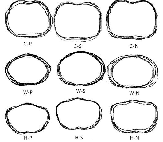
Table 3-5 show that, the absolute error of calculating CWH are respectively in (–1.47 cm~1.44 cm), (–1.50 cm~1.51 cm), (–1.60 cm~1.63 cm), which basically meet the requirement of ±1.5 cm in garment industry. The errors caused by the measuring and calculating process are improved as follows. Overlap and piece the 4-5 groups of curve figures of the largest positive and negative error and the minimal absolute error, as Fig. 11 shown. It can be seen that, curves of the lager positive error- P model, the negative error- N model and the smaller absolute error- S model have the similar traits in shape and trend. Classify CWH curves in the above cross-section shapes in advance, using image recognition. Calculate the intercept $B$ with different regression formulas for different types of curves, and then run the integrations. This process can decrease the error effectively.

The results and the comparisons between the calculating circumference s and the measuring circumference s of the static and dynamic experiments, in which all the subjects wear different daily clothes and their body shape were classified in advance, are shown in Table 6 and Table 7.

Table 6 shows that, different dressings have some impacts on the selection of the feature points and the circumference calculation of the fitted curves. When the subjects wear clothes of soft textured and elastic fabric, whose styles highlight the body curves and fit, the errors of the measuring experiment are less.

Table 7 shows that, although the information of the featured points captured from the subjects’ walking state is different, the $CWH$ calculated vales are less different, which can meet the industry requirement. Certainly, the function of binding bands is not ignored, but as the feasibility discussion of the method, this experiment provides a possibility. And it should be studied how to get rid of the $CWH$ binding bands and obtain the featured points’ data in the future practical application.

Fig. 11Actual CWH cross-section curves of different error type

6. Conclusions

Comparing the length dimension which can be obtained more easily, how to generate the $CWH$ girth using limited feature points is one of the main subjects in the field of 2D-3D non-contact anthropometry used for garment industry. Taking Asian young women as researching objects, by regression analysis and curve fitting, algorithms of the $CWH$ circumferences were presented in this paper. As for the daily dressing state and the dynamic measuring mode, representative experiments were conducted, which had guidance meaning for making non-contact body measurement more convenient. By extracting the feature points in natural wearing state, static and dynamic, and using the algorithms mentioned above, the $CWH$ measurements were well obtained. This process is effective and provides a foundation for the rapid shape recognition and classification.