An intelligent fault diagnosis method of rotating machinery using L1-regularized sparse filtering

1. Introduction

With the rapid development of technology, industrial Internet of Things (IoT) and data driven techniques [1] have been revolutionizing manufacturing. As machines are becoming more efficient and automatic than ever before, it is more significant to have a safe and sound operation [2]. Meanwhile, rotating speed oscillation usually occurs during machine operation which can accelerate the damage on machines [3]. Therefore, condition monitoring systems are adopted to collect the massive amount of data from monitored machines [4, 5]. At the same time, with substantial development of computing systems and sensors, machinery fault diagnosis has fully embraced the extensive revolution in modern manufacturing.

Traditionally, there are mainly three sequential steps in the framework of fault diagnosis systems: 1) signal acquisition; 2) feature extraction and selection and 3) fault classification [2, 6, 7]. In the first step, vibration signals are widely used as the data source since essential information about machine health condition is embedded in them. However, feature extraction is always needed because the raw signals contain various kinds of noise. In the second step, representative features are extracted for fault classification. The more discriminative features are extracted from vibration signals, the more accurate fault diagnosis result would be. Signal processing techniques have been proposed and widely used in feature extraction and selection such as time-domain analysis [8], frequency transform [9], high resolution time-frequency analysis [10], wavelet transform [11], and envelope demodulation algorithms [12]. Besides, as entropy is effective in detection the dynamic characteristics of time series, some methods use entropy in feature extraction and selection. Modified multi-scale symbolic dynamic entropy (MMSDE) [13] and modified hierarchical permutation entropy (MHPE) [14] were proposed to extract features for gearbox fault diagnosis. Zhao et al. [15] combined the EEMD and multi-scale fuzzy entropy to extract more discriminative features. However, the further analysis of features extracted by these algorithms requires manpower and prior knowledge. At the same time, although these techniques can effectively extract primary features from signals, these features may prevail among all signals of various health conditions. Therefore, dimension-reduction strategies such as nonlinear PCA [16], independent component analysis (ICA) [17] are required to select sensitive features. It means that these extracted features should be sensitive to different health conditions but be insensitive to different operating conditions such as large speed oscillation. Intelligent feature learning methods can also be utilized in feature extraction along with feature selection. Among various intelligent feature learning methods, unsupervised ones have been successfully applied to extract useful features in many image, video and audio tasks.

Well developed as unsupervised feature learning algorithms are, there are still two main drawbacks [18]. Firstly, unsupervised learning algorithms generally have plenty of parameters, which are difficult to tune and crucial to the performance of the network. The comparison of tunable parameters in various unsupervised learning algorithms is shown in Table 1 [18, 19]. It can be seen that there are massive parameters in sparse restricted Boltzmann machines (RBMs) [20], sparse autoencoder [21], sparse coding [22]. Secondly, computational complexity is also a major drawback. Independent component analysis (ICA) has just one hyperparameter needing tuning [23] and provides commendable results in object recognition experiments, but it scales poorly to large datasets and high-dimension inputs. Sparse coding has an expensive inference process, which requires a costly optimizing iteration. Stacked autoencoder (SAE) [24] has to do a greedy layer-wise training process which includes decoding and encoding networks, and the parameters of decoding network are useless in fine tuning which will increase the computational complexity. In the final step, the learned features are utilized to train the classifiers such as support vector machine (SVM) and softmax regression [25], which are always used to identify the health condition. In Ref. [26], the improved Particle Swarm Optimization (PSO) algorithm was proposed to optimize the parameters of least squares support vector machines (LS-SVM) in order to construct an optimal classifier.

As sparsity is one of the desirable properties of a good feature representation [27], Ngiam et al. [19] proposed an unsupervised algorithm called sparse filtering to solve the problems pointed out above, which is a two-layer neural network. Only the dimension of features learned from sparse filtering needs tuning and its main idea is the sparsity of the feature matrix [18]. Meanwhile, it was validated on image recognition and phone classification tasks, which obtained the state-of-the-art performance. For its simplicity and good performance, Lei et al. [2] introduced sparse filtering into rotating machine fault diagnosis and constructed a two-stage intelligent fault diagnosis method, which got better performance than other networks. Sparse filtering works by imposing sparse constraints on the distribution sparsity of the feature matrix but the overefitting risk of it is quite high, namely having poor generalization ability. Yang et al. [28] utilized L2 norm to regularize the weight matrix of sparse filtering. However, its effectiveness in preventing overfitting is limited and it takes no consideration of the sparsity of the weight matrix. Meanwhile, the activation functions used in weight matrix optimization of sparse filtering [2] are soft-absolute function, which computes fast and can partly avoid the gradient vanishing problem. Nevertheless, when it is used in feedforward, its robustness to noise is weak. L1 norm can also be utilized to reduce the overfitting risk. However, when introducing L1 regularization into the original network, the optimization of the new network is difficult sometimes. Recently, Deng et al. [29, 30] introduced new algorithms into solving complex optimization problems, which can be beneficial to the network with many terms to be optimized. With the help of them, L1 norm can be utilized better.

Inspired by Ref. [28-30], aiming at reducing the overfitting risk, an improved sparse filtering network with L1 regularization is proposed, which can improve the performance of the network by exploring the sparsity of the weight matrix. Meanwhile, for considering the different requirements of non-saturating and anti-noise properties, we propose using different activation functions in feature extraction network training and feedforward, which is inspired by the training process of deep learning that different activation functions can be adopted in greedy layer-wise pre-training and further fine tuning.

The main contributions of this paper are described as follows:

(1) A three-stage intelligent fault diagnosis method of rotating machinery is developed. In the first stage, time-domain samples are automatically pre-processed into frequency-domain samples by FFT. In the second stage, an improved feature extraction network called L1-regularized sparse filtering is proposed to extract and select discriminative features. In the last stage, features are fed into softmax regression to identify the health condition. Experiments conducted on a bearing dataset and a gearbox dataset verify the effectiveness of the proposed method.

(2) L1-regularized sparse filtering is proposed to constrain the weight matrix sparsity and improve the generalization ability of standard sparse filtering. We also construct the L2-regularized sparse filtering and do experiments on it. The comparison with standard sparse filtering demonstrates its effectiveness. The comparison with L1-regularized sparse filtering shows it is inferior when using frequency-domain samples.

(3) An interpretation of the weight matrix learned by sparse filtering is given, which is the supplement to the interpretation given in Ref. [2]. Based on it, two sparse properties of the weight matrix are defined, which are validated significant in obtaining discriminative features. They also explain why L1-regularized sparse filtering performs better when frequency-domain samples are adopted.

This paper is organized as follows. Section 2 describes sparse filtering and L1 regularization briefly. Section 3 details the proposed L1-regularized sparse filtering and the using of the new activation function. In Section 4, diagnosis cases of a bearing dataset and a gearbox dataset are studied separately using the proposed method and other models. Section 5 discusses the properties of the weight matrix learned by the improved sparse filtering. Finally, the conclusion is drawn in Section 6.

2. Theoretical background

2.1. Sparse filtering

Generally, unsupervised feature learning algorithms can be divided into two main categories [18]: explicitly modeling the input distribution or not. ICA, sparse coding, SAE and sparse RBMs explicitly model the input distribution and reconstruct mechanical dynamic signal structure by minimizing the reconstruction error. Although it’s desirable to learn a good approximation of the input distribution, algorithms such as sparse filtering show that this is not so important if the aim is to get discriminative features. The fundamental idea of sparse filtering focuses on constraining the sparsity of output features instead of explicitly modeling the input distribution. Sparse filtering tries to learn sparse feature distribution that satisfies three principles:

(1) Population sparsity, which refers that all the features of one sample should be activated sparsely at a time;

(2) Lifetime sparsity, which refers that the same kind of features belonging to all samples should be activated sparsely at a time;

(3) High dispersal, which refers that all kinds of features should have similar statistics.

The architecture of the sparse filtering network is shown in Fig. 1. Firstly, the collected raw vibration data is alternately separated into $K$ samples. Then they are transformed from original time-domain samples into Fourier spectra $\{{\mathbf{x}}^i{\}}_{i=1}^K$ by fast Fourier transformation (FFT), where ${\mathbf{x}}^i\in R^{N\times 1}$ is $i$th sample containing $N$ Fourier coefficients, which are the amplitudes of the spectral lines. Next, the training dataset is used to train sparse filtering to get an optimized weight matrix $\mathrm{W}\in R^{N\times N^{out}}\text{,}$ where $L$ is the dimension of output feature vectors. Finally, the frequency-domain sample ${\mathbf{x}}^i\in R^{N\times 1}$ is mapped into a feature vector ${\text{f}}^i\in R^{N^{out}\times 1}$ in feedforward. The mapping can be realized through $\mathbf{W}$ and activation function 2.

Fig. 1Architecture of the sparse filtering network

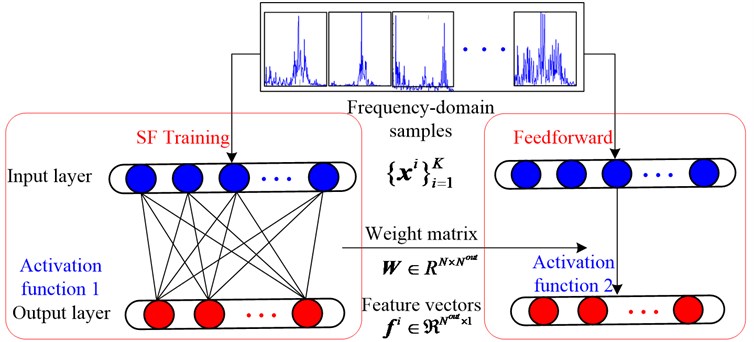
In the optimization, the standard sparse filtering uses a soft-absolute function as activation function 1 [19], so the features can be computed as follows:

1

$f_j^i=\sqrt{\epsilon +{\left({\mathbf{W}}_j^T{\mathbf{x}}^i\right)}^2}\approx \left|{\mathbf{W}}_j^T{\mathbf{x}}^i\right|,$

where $f_j^i$ refers to the $j$th feature of the $i$th sample and $\epsilon$ is set to 10^-8. The feature matrix learned from training dataset is $\mathbf{f}\in R^{N^{out}\times K}$, where $K$ is the number of training samples and $N^{out}$ is the dimension of output feature vectors. Three steps should be applied to realize the sparse principles mentioned above, which are shown as follows.

Firstly, by means of dividing each kind of feature using its L2 norm [2] across all samples, each kind of feature ${\mathbf{f}}_j$ is normalized to be equally active:

2

${\tilde{\mathbf{f}}}_j=\frac{{\mathbf{f}}_j}{{‖{\mathbf{f}}_j‖}_2},\mathrm{}\mathrm{}\mathrm{}\left(j=\mathrm{1,2},\dots ,N^{out}\right).$

Then, the new feature matrix is normalized by columns, so that features of each sample ${\tilde{\mathbf{f}}}^i$ lie on the unit L2 ball:

3

${\widehat{\mathbf{f}}}^i=\frac{{\tilde{\mathbf{f}}}^i}{{‖{\tilde{\mathbf{f}}}^i‖}_2},\mathrm{}\mathrm{}\mathrm{}\left(i=\mathrm{1,2},\dots ,K\right).$

At last, the normalized features are optimized for sparsity by L1 norm. The objective function of sparse filtering can be described as follows:

4

$\underset{\mathbf{W}}{\mathrm{m}\mathrm{i}\mathrm{n}\mathrm{i}\mathrm{m}\mathrm{i}\mathrm{z}\mathrm{e}}\sum _{i=1}^K{‖{\widehat{\mathbf{f}}}^i‖}_1=\sum _{i=1}^K{‖\frac{{\tilde{\mathbf{f}}}^i}{{‖{\tilde{\mathbf{f}}}^i‖}_2}‖}_1.$

In this paper, we take a novel view on sparse filtering: considering it as a greedy layer-wise training process [31], which means that the activation function used in fine-tuning process could be different from the one used in weight matrix initialization and that is analogous to the training process in SAE. Therefore, to get a more noise-robust feature representation, we adopt Eq. (5) as activation function 2:

5

${\mathbf{f}}_j^i=\mathrm{l}\mathrm{o}\mathrm{g}\left(1+({\mathbf{W}}_j^T{\mathbf{x}}^i{)}^2\right),$

instead of the widely used soft-absolute function, as shown in Fig. 1.

3. Proposed framework

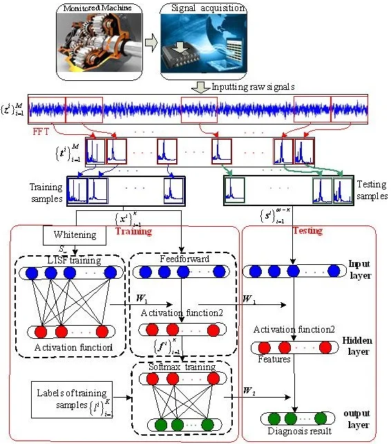
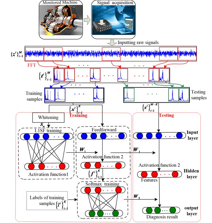
This section details how the proposed method automatically extracts features from raw data and then briefly describes how the diagnosis results are obtained. The framework of our method is illustrated in Fig. 2 and the process can be described as follows.

(1) Data sampling and preprocessing. The time-domain raw signals are sampled into dataset $\{{\mathbf{z}}^i{\}}_{i=1}^M$, where ${\mathbf{z}}^i\in R^{2N\times 1}$ is the $i$th sample containing $2N$ data points. Then each sample ${\mathbf{z}}^i$ is transformed into frequency-domain sample ${\mathbf{t}}^i$ by FFT, where ${\mathbf{t}}^i\in R^{N\times 1}$ is the $i$th sample containing $N$ Fourier coefficients. These samples are combined into dataset ${\left\{{\mathbf{t}}^i\right\}}_{i=1}^M$.

(2) Training dataset selection and whitening. $K$ samples are randomly selected from ${\left\{{\mathbf{t}}^i\right\}}_{i=1}^M$ composing the training dataset ${\left\{{\mathbf{x}}^i\right\}}_{i=1}^K$ and the label set of the training samples is ${\left\{l^i\right\}}_{i=1}^K$, where $l^i$ is the label of sample ${\mathbf{x}}^i$. The rest samples compose the testing dataset ${\left\{{\mathbf{s}}^i\right\}}_{i=1}^{M-K}$. A whitening approach [2] is utilized to preprocess the training samples and obtain the whitened dataset ${\mathbf{S}}_w\in R^{N\times K}$, where $K$ is the number of samples and $N$ is the dimension of samples.

(3) Sparse filtering training. Firstly, the whitened dataset ${\mathbf{S}}_w$ is fed into the L1-regularized sparse filtering model. Then, the weight matrix ${\mathbf{W}}_1\in R^{N\times N^{out}}$ is obtained by minimizing the new objective function as Eq. (6), where $N^{out}$ is the output dimension. It should be noted that Eq. (1) is used as activation function 1.

(4) Output features calculation. A feedforward process is carried out on the training dataset ${\left\{{\mathbf{x}}^i\right\}}_{i=1}^K$ with the optimized weight matrix ${\mathbf{W}}_1$ and activation function 2. The new function described in Eq. (5) is adopted as activation function 2. Each sample ${\mathbf{x}}^i$ is mapped into feature vector ${\mathbf{f}}^i\in R^{N^{out}\times 1}$, so the feature matrix of training samples is ${\left\{{\mathbf{f}}^i\right\}}_{i=1}^K$.

(5) Softmax regression training. The feature matrix ${\left\{{\mathbf{f}}^i\right\}}_{i=1}^K$ together with the labels of the training samples ${\left\{l^i\right\}}_{i=1}^K$ is fed into the softmax regression to train the network. The trained softmax regression will be used to identify the health conditions of feature vectors.

(6) Diagnose the testing samples. The trained network is employed to identify health conditions of testing samples${\left\{{\mathbf{s}}^i\right\}}_{i=1}^{M-K}$, as shown in Fig. 2.

Fig. 2Flowchart of the proposed method

4. Fault diagnosis using the proposed method

In this section, a bearing dataset and a gearbox dataset are employed to validate the effectiveness of our method. In order to further verify the superiority of our method, six different networks are constructed, as shown in Table 2, where SF denotes sparse filtering; L1SF denotes L-regularized sparse filtering; L2SF denotes L2-regularized sparse filtering. Meanwhile, 20 trials are carried out for each experiment to reduce the effect of randomness. The parameters are all tuned to the best, and the regular parameter of softmax regression is tuned to 1E-5 [2]. The computation platform is a PC with an Intel I5 CPU and 8G RAM.

4.1. Case 1. Fault diagnosis of rolling element bearings

4.1.1. Data description

The motor bearing experimental dataset provided by Case Western Reserve University [34] is employed in this section. The vibration signals were collected from the drive end of the motor through the tri-axial accelerator. The dataset contains four different health conditions: 1) normal condition (NC); 2) outer race fault (OF); 3) inner race fault (IF) and 4) roller fault (RF). Vibration signals of three different damage severity levels (0.07, 0.14 and 0.21 inch) were separately collected for health condition OF, IF and RF. In addition, the signals were all collected under three different loads (1, 2 and 3 hp) and the sampling frequency was 48 kHz. The total dataset is composed of ten health conditions under three loads, and we treat the same health condition under different loads as the same class. 300 samples are obtained from each health condition under one load, so the dataset is composed of 9000 samples and each sample includes 1600 time-domain data points.

4.1.2. Parameter selection and diagnosis result

In this subsection, the dataset will be processed by the proposed method. Firstly, FFT is implemented on each time-domain sample and 1600 Fourier coefficients are obtained. As the coefficients are symmetric, we utilize the first 800 coefficients in each sample, so each sample contains 800 Fourier coefficients. As there is no obvious periodic property in each frequency-domain sample, the coefficients of each sample are treated as a whole. Therefore, there is no need to segment it in the way mentioned in Ref. [2] and the dataset ${\left\{{\mathbf{x}}^j\right\}}_{j=1}^{9000}$ is used to train and test the network, where ${\mathbf{x}}^j\in R^{800\times 1}$.

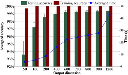
First, we investigate the selection of the parameters of sparse filtering. We randomly select 10 % of samples to train the proposed method and the rest of the samples are used for testing. The averaged diagnosis results of L1SF-LOG with different output dimensions are shown in Fig. 3. It presents that the testing accuracy is higher than 99.2 % when $N^{out}$ is bigger than 600. It is evident that the testing accuracy goes higher and the corresponding standard deviation drops continuously with the increase of $N^{out}$, but the averaged training time keeps increasing. It indicates that we should make a tradeoff between the diagnosis accuracy and the time spent while selecting $N^{out}$. It can be seen that the increase of accuracy is unobvious when $N^{out}$ is bigger than 700, so we choose 700 as $N^{out}$. The testing accuracy reaches the highest and the standard deviation reaches the lowest when the regular parameter of L1SF-LOG is around 100, so it is set to 100, as displayed in Fig. 4. The output dimension and regular parameter of L2SF-LOG are tuned to 400 and 10 respectively. The output dimensions of SF-LOG and SF-ABS are tuned to 700 and 100 separately.

Fig. 3Output dimension selection

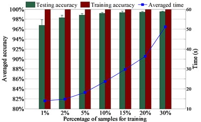
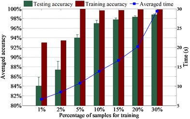
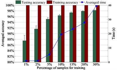
The diagnosis results using various numbers of samples for training are presented in Fig. 5. It presents in Fig. 5(a) that the testing accuracy rises moderately with the increase of training sample number because the testing accuracy is higher than 96 % with just 1 % samples for training. Fig. 5(a) also shows that L1SF-LOG can diagnose ten health conditions with averaged testing accuracy up to 98 % when only 2 % samples are used for training, and the testing accuracy rises to 99 % when the percentage of training samples increases to 5 %. At the same time, it can be observed from Fig. 5 that the test accuracy is up to 96 % when the training samples for L2SF-LOG, SF-LOG, and SF-ABS increase to 10 %, 10 % and 20 % respectively. It indicates that L1SF-LOG can achieve excellent performance even while lacking training samples and L1SF-LOG performs better than L2SF-LOG.

Fig. 4The regular parameter of L1SF-LOG

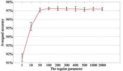
Fig. 5Diagnosis results of: a) L1SF-LOG, b) L2SF-LOG, c) SF-LOG, d) SF-ABS with different percentage of training samples

a)

b)

c)

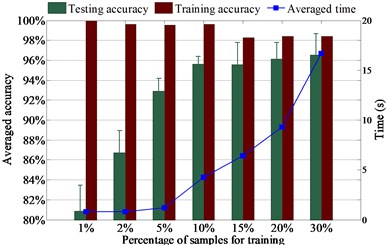
d)

It also indicates in Fig. 5 that L1SF-LOG can prevent the overfitting dramatically since the gaps between training accuracy and testing accuracy are always smaller than 3.7 %. By comparison, it shows that L1SF-LOG and L2SF-LOG both have higher testing accuracies and smaller gaps between training accuracy and testing accuracy than SF-LOG under the same training sample number. Meanwhile, it also presents that SF-LOG outperforms SF-ABS, which benefits directly from the using of the new activation function. Furthermore, when using same numbers of samples in training, L1SF-LOG always holds the lowest standard deviation, which indicates L1SF-LOG is more stable than the other three networks. In the following experiments, we randomly select 15 % samples from the whole dataset for training.

To further present the efficiency of the proposed method, 20 trials averaged accuracies and their standard deviations of all the six networks are shown in Table 3. It shows that L1SF-LOG holds the highest accuracy and lowest standard deviation, which means L1SF-LOG is more stable than the others. Meanwhile, it is worth mentioning that SF-LOG performs better than SF-ABS. Comparing the results of SF-LOG and SF-ABS, L2SF-LOG and L2SF-ABS, L1SF-LOG and L1SF-ABS, it presents that the networks which adopt the new activation in feedforward can achieve higher testing accuracies and are much more stable.

The 20 trials averaged confusion matrix of L1SF-LOG shows that the health conditions IR7 and OR7 will be misclassified as each other most probably, as displayed in Table 4. It can be assumed that the health conditions misclassified as each other, mainly because signals of them are similar to each other. The normal health condition is classified perfectly mainly because it has no fault and is most distinct from other health conditions.

Table 3The setting and performance of 6 networks

Method	Output dimension	Training accuracy (%)	Testing accuracy (%)	Training time (s)
SF-ABS	100	98.26±2.94	95.57±2.21	6.41±0.34
SF-LOG	700	100	97.37±0.27	23.30±0.58
L1SF-LOG	700	100	99.39±0.23	29.84±0.39
L2SF-LOG	400	99.73±0.27	97.61±0.27	16.68±0.38
L1SF-ABS	700	99.50±0.68	98.08±0.89	25.30±1.06
L2SF-ABS	700	99.49±0.24	97.23±0.42	23.30±0.74
Note: The format of the result is: mean value ± standard deviation

Table 4Confusion matrix of 20 trials averaged diagnosis results

Predict true	NOR	BALL7	BALL14	BALL21	IR7	IR14	IR21	OR7	OR14	OR21
NOR	765	0	0	0	0	0	0	0	0	0
BALL7	0	765	0	0	0	0	0	0	0	0
BALL14	0	0	761.65	0	0	0.15	3.2	0	0	0
BALL21	0	0	0	764.85	0	0	0	0	0	0.15
IR7	0.25	1.85	0.15	0.7	748.9	3.45	0	1.05	6.15	2.5
IR14	0	0	0	0	1.1	760.3	0.3	0	3.25	0.05
IR21	0	0	4.25	0.25	0.1	1.05	759.3	0	0.05	0
OR7	0	0	0	0	1.4	0	0	763.2	0.15	0.25
OR14	0	0	0.7	0.1	13.9	1.3	0.1	1.05	747.8	0.05
OR21	0	0.85	0.5	1.15	0.05	0.4	0	0	0	762.05

4.2. Case2. Fault diagnosis of gearbox

4.2.1. Data description

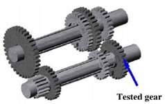
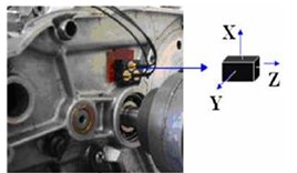
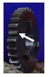
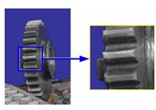
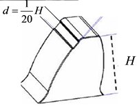
The vibration signals of a four-speed motorcycle gearbox [35] used in this section were collected from the test rig as shown in Fig. 6. The test rig was also equipped with a tri-axial accelerometer, a data acquisition system, a load mechanism, an electrical motor, a tachometer and four shock absorbers. The vibration signals of four conditions were collected: 1) normal condition (NC); 2) medium-worn (MW); 3) broken-tooth (BT) and 4) slight-worn (SW), as shown in Fig. 6 and each health condition has one load. The sampling frequency was 16384 Hz. 80 samples are sampled for each health condition from raw data, where each time-domain sample contains 800 data points.

Fig. 6a) test rig, b) schematic of the gearbox, c) accelerometer location, d) broken teeth defect, e) worn teeth defect, f) worn model defect

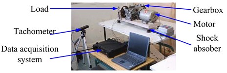
a)

b)

c)

d)

e)

f)

4.2.2. Diagnosis result

The preprocessing of each sample is the same as the bearing case, 400 Fourier coefficients are obtained from each sample. 10 % samples are randomly selected for training and the rest for testing. The output dimensions $N^{out}$ for experiments of various networks are all tuned to 400 and the regular parameters ${\lambda }_1$, ${\lambda }_2$ are all tuned to 100.

Fig. 7Diagnosis results of 20 trials

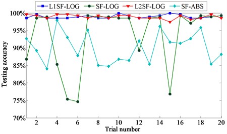
20 trials are carried out for each experiment, and the comparison of diagnosis results among 4 networks is depicted in Fig. 7. It shows that the averaged accuracies are mostly over 99.5 % for L1SF-LOG and 99.0 % for L2SF-LOG, and both of them also hold quite low accuracy fluctuations. By comparison, it indicates that the new activation function can extract better features than the soft-absolute function, and L1 regularization is effective in improving the performance of standard sparse filtering.

Table 5Training and testing accuracies of 6 networks

Method	Training accuracy (%)	Testing accuracy (%)
SF-ABS	100	88.35±7.85
SF-LOG	100	94.51±6.19
L1SF-LOG	100	99.13±0.50
L2SF-LOG	100	98.80±0.56
L1SF-ABS	100	94.82±4.24
L2SF-ABS	100	98.05±0.61
Note: The format of the result is: mean value ± standard deviation

To quantitatively show the efficiency of L1SF-LOG and L2SF-LOG in preventing overfitting, the averaged accuracies and standard deviations of each network are shown in Table 5. It shows that the improved networks all perform better than SF-ABS, and L1SF-LOG holds the highest classification accuracy and the lowest standard deviation once again. Meanwhile, it also presents that the difference between averaged training accuracy and testing accuracy of L1SF-LOG is the smallest, namely 0.87 %. Furthermore, it is worth mentioning that the standard deviation is 0.5 % for L1SF-LOG and 0.56 % for L2SF-LOG, which means L1SF-LOG and L2SF-LOG are stable, and L1SF-LOG is superior to L2SF-LOG.

5. Discussion

Experiments on these networks show that proposed L1SF-LOG can obtain much higher testing accuracy, stability and generalization ability than the others, and networks with the new activation function perform better than the ones without. It also demonstrates that although inferior to L1-regularized sparse filtering, the L2-regularized sparse filtering is also effective in improving some aspects of performance.

We focus on the process of feature calculation and investigate why L1SF-LOG holds the best performance. As sparse filtering has no bias term, if we use $F\left(x\right)=x$ as the activation function, then we can describe the feature calculation process as follows:

Fig. 8Columns and rows of weight matrices learned from the bearing dataset: a) L1SF-LOG, b) L2SF-LOG, c) SF-LOG

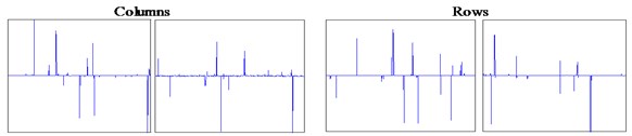
a)

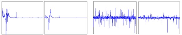
b)

c)

We regard each column of $\mathbf{W}$ as a filter [2] and the features are extracted by the inner product of weight matrix columns and sample ${\mathbf{x}}^i$. When samples are fixed, we want the filters to extract discriminative features and do not want these features to be extracted repeatedly, which means that the sparsity of the weight matrix should be ensured in a certain degree. Heuristically, as sparse filtering achieves the sparsity of the feature matrix by implementing L1 norm in the objective function, we utilize L1 regularization to constrain the sparsity of the weight matrix. Similarly, when the samples are frequency spectra, we propose defining the population sparsity and lifetime sparsity of weight matrix as follows:

(1) Population sparsity, which refers that the columns of the weight matrix have very narrow passing bandwidths. It should be noticed that different from common filters, each column of the weight matrix can have several main lobes, which means that it can fuse several weakly discriminative features by composing them into a prominent one.

(2) Lifetime sparsity, which refers that the rows of the weight matrix should be sparsely activated, which means the same frequency band will not be filtered repeatedly. It prevents the discriminative features from being extracted by many times and reduces the information redundancy in feature representation. As a result, more discriminative features are mined.

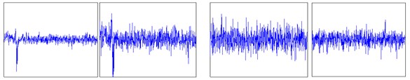
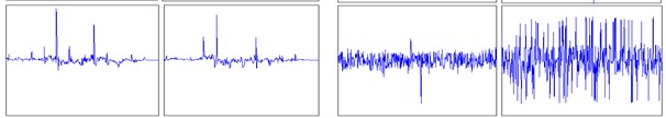
To further present the effectiveness of sparsity in the weight matrix, typical rows and columns of weight matrices learned from L1SF-LOG, L2SF-LOG, SF-LOG are presented in Fig. 8 and Fig. 9. Firstly, it can be seen that all the columns of weight matrix learned by each network serve as band-width filters for frequency-domain samples and the ones learned by L1SF-LOG have the best frequency-domain filtering property. By comparison, it can be concluded that L1SF-LOG holds this property because its weight matrix is constrained by L1 regularization. Secondly, it also presents that the columns and rows of weight matrices learned by L1SF-LOG are all highly sparse, which means that the weight matrix has the population sparsity and lifetime sparsity defined above. Therefore, it is validated that L1 regularization is effective in constraining the sparsity of the weight matrix in sparse filtering. Furthermore, it can also be found that the columns of weight matrix learned by L2SF-LOG are smoother than SF-LOG.

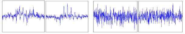
Fig. 9Columns and rows of weight matrices learned from the gearbox dataset: a) L1SF-LOG, b) L2SF-LOG, c) SF-LOG

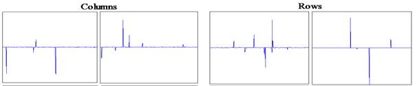
a)

b)

c)

6. Conclusions

A new feature extraction method called L1-regularized sparse filtering is proposed to extract more discriminative features and improve generalization ability of standard sparse filtering through constraining the sparsity of the weight matrix. Based on FFT, L1-regularized sparse filtering and softmax regression, a novel three-stage fault diagnosis method is developed. Experiments on a bearing dataset and a gearbox dataset demonstrate that L1SF-LOG is more effective in preventing overfitting than L2SF-LOG, SF-LOG and SF-ABS. Meanwhile, the proposed L1SF-LOG can obtain much higher diagnosis accuracy with less training samples and be more stable.

We propose adopting different activation functions in feedforward and weight matrix optimization for considering their different requirements of anti-noise and non-saturating properties. Experiments show that this operation improves the testing accuracy and the diagnosis network stability a lot. Furthermore, we give an interpretation of the weight matrix and define two sparse properties of weight matrix. The significance of the two properties is validated by experiments. It shows that the weight matrix learned by L1SF-LOG has the sparse properties described above, which accounts for its superiority.