A new highly anti-interference regularization method for ill-posed problems

1. Introduction

In engineering technologies, there are a large amount of inverse problems in mathematical physics from different fields, such as seismic exploration, image processing, load identification, and so on. In most cases, the inverse problems of mathematical physics are ill-posed, and a large amount of ill-posed problems can be transformed into the first kind Fredholm integral equations, which can be discretized into a system of linear algebraic equations, and by solving it the solution of the problem of mathematical physics can be obtained. However, the discretized algebraic equations are normally also ill-posed. So, the regularization methods for solving this kind of problems have become the focus in this research field, in which the selection of regularization parameters has gotten much attention.

The research of regularization theory and method for ill-posed problems can be traced back to 1923, when one of the world’s most famous mathematicians Hadamard conducted a study and gave a description of ill-posedness of the Cauchy problem of linear partial differential equations. In the 1940s, Tikhonov an academician of the former Soviet Union started to systematically study the theories and methods of ill-posed problems, and a widely used Tikhonov regularization method was put forward. Then a very classical monograph, Solutions of Ill-Health Problems, was published in the 1970s. Since then many researchers have devoted to the research and put forward different forms of regularization methods. This paper presents a new regularization method after a careful study of the existing regularization methods. So, let us start with the equation that we are going to solve:

Let $\mathbf{X}$ and $\mathbf{Y}$ be Hilbert Spaces, $\mathbf{K}\in L\left(\mathbf{X},\mathbf{Y}\right)$, where $\mathbf{K}:\mathbf{X}\to \mathbf{Y}$ is a bounded continuous linear operator [1, 2]. We discuss the typical mathematical expression of linear inverse problems consisting in the solution of linear operator equation:

Eq. (1) is usually an ill-posed problem, i.e. the solution of problem need not be unique or does not depend continuously on the right-hand side, and the second situation is discussed in most cases, which means that if the data on the right hand side have small perturbations, large deviations of the solution will appear. The data $\mathbf{y}$ in Eq. (1) has perturbations, the expression of the distorted data can be expressed as:

where $\mathbf{\tau }$ is a diagonal matrix with random elements coming from [–1, 1], $\delta$ is the indicator of perturbation.

The core of the article is how to solve the following equation effectively:

and establishing an effective regularization method is the key task.

This article is organized as follows: In Section 2, we propose a new regularization filter and the related new regularization method and prove its rationality. In Section 3, we give an accuracy estimate of the solution and present a method for the selection of regularization parameters for the new regularization method. In Section 4, we test the new regularization method by solving the first kind Fredholm integral equation and demonstrate the stability and validity of the new regularization method.

2. Construction of new regularization method

The existing regularization methods are mostly based on the perturbation theory and the continuation method, and typical representatives are the Tikhonov regularization method, the iterative methods, and other improved methods. In this section, we propose a new filter factor and correspondingly establish a new regularization method. In addition, we prove that the new regularization method is valid from the view of mathematics.

The Tikhonov regularization method is composed of the following filter factor:

where $\alpha$ is a regularization parameter, $\mu$ is the singular value of matrix $\mathbf{K}$.

The solution of Eq. (3) with Tikhonov regularization method can be expressed as:

We define a new filter factor $q$($\alpha$, $\mu$) as follows:

Theorem 2.1 If $q$($\alpha$, $\mu$) is a filter factor given by Eq. (6), we have [3-5]:

1) $0<q\left(\alpha ,\mu \right)<1$, $\alpha >0$, $\mu \in \left(\left.0,‖\mathbf{K}‖\right]\right.$;

2) $\underset{\alpha ⟶0}{\lim }q\left(\alpha ,\mu \right)=1$, $\mu \in \left(\left.0,‖\mathbf{K}‖\right]\right.$;

3) $q\left(\alpha ,\mu \right)<\frac{\pi }{2\alpha }\mu$, $\alpha >0$, $\mu \in \left(\left.0,‖\mathbf{K}‖\right]\right.$;

4) $1-q\left(\alpha ,\mu \right)\le \frac{{\pi }^2\alpha }{8\mu }$, $\alpha >0$, $\mu \in \left(\left.0,‖\mathbf{K}‖\right]\right.$.

Proof obviously, 1) and 2) are valid, so we only need to prove 3) and 4).

3) It is easy to know that $\mathrm{s}\mathrm{i}\mathrm{n}（a）<a$ and $0<a<1$, so we have:

4) We prove this conclusion in two different situations:

When:

When:

According to Theorem 2.1, we are sure that Eq. (6) is a reasonable regularizing filter, and the approximate solution of Eq. (3) can be defined as:

where $R_{\alpha }:\mathbf{Y}\to \mathbf{X}$ is defined as follows:

The corresponding formula for solving Eq. (3) is as follows:

where $\mathbf{\beta }$ is a vector with the elements the correction factors.

3. Optimum selection of the regularization parameters

In order to obtain a stable and accurate approximate solution of Eq. (3), some regularization methods are usually adopted. The regularized approximate solution ${\mathbf{x}}_{\alpha }^{\delta }=R_{\alpha }*{\mathbf{y}}^{\delta }$ has the nature: when $\delta \to 1$, ${\mathbf{x}}_{\alpha }^{\delta }\to \mathbf{x}$, where the regularization parameter $\alpha =\alpha \left(\delta \right)$ must be properly selected. In this way, the regularization solution ${\mathbf{x}}_{\alpha }^{\delta }$ can continuously depends on the right hand side data of Eq. (3). In general, if the unknown solutions of ill-posed problems are not confined to a certain range, the regularization solution ${\mathbf{x}}_{\alpha }^{\delta }$ may converge to the real solution $\mathbf{x}$ very slowly. In order to get a faster convergence rate of ${\parallel \mathbf{x}}_{\alpha }^{\delta }-\mathbf{x}\parallel$, the approximate solutions of Eq. (3) need to be restricted to some source collections. We define a subspace of $\mathbf{X}$:

where:

Thus, we can give an accurate estimate of the solution error by using the following theorem.

Theorem 3.1 Assume that the following conditions are met:

a) $\parallel {\mathbf{y}}^{\delta }-\mathbf{y}\parallel <N$, where $N$ is a constant;

b) $\mathbf{K}:\mathbf{X}\to \mathbf{Y}$ is a compact linear operator and injective one-to-one, $\mathbf{y}\in R（\mathbf{K}）$;

c) ${\mathbf{M}}_{\alpha ,E}=\left\{\mathbf{x}\in \mathbf{X}:{\parallel \mathbf{X}\parallel }_{\alpha }\le E\right\}$, the source condition $\mathbf{x}\in M_{\alpha ,E}$ is required.

Then we have:

Proof: According the triangle inequality, we have:

Using the properties of singular system of $\mathbf{K}$ and Eqs. (3), (4) in theorem 2.1, we obtain:

So, we have the error estimate Eq. (16) and now we need to know how to get the suitable values of its regularization parameters.

For actual engineering problems, the prior information of the solution is generally unavailable. Thus, it is difficult or impossible to determine a suitable value for the regularization method, and the error to the actual measurement is unknown. In this case, the L-curve method is often used to select the proper regularization parameters [6, 7]. If the proper regularization parameters are selected by the L-curve method, it is possible to achieve an optimal asymptotic convergence rate in the iterative calculation. Based on the L-curve method [6, 7], we use the ergodic searching to find the proper regularization parameters, i.e. to ensure that the sum of absolute value of $\left(\mathbf{K}{\mathbf{x}}_{\alpha ,\beta }^{\delta }-{\mathbf{y}}^{\delta }\right)$ is as small as possible. In other words, we need to try as much as possible combinations of the regularization parameters ($\alpha$, $\beta$) to find the smallest value in all those sums of absolute value of $\left(\mathbf{K}{\mathbf{x}}_{\alpha ,\beta }^{\delta }-{\mathbf{y}}^{\delta }\right)$ and the corresponding combination of regularization parameters ($\alpha$, $\beta$) is just the suitable values for the new regularization method.

4. Numerical tests

In order to demonstrate the stability and validity of the new regularization method proposed in this article, we now test the method by solving the first kind Fredholm integral equation. The first kind Fredholm integral equations are usually ill-posed, and when the Fredholm integral equation is discretized into a linear algebraic equation, the matrix equation is also ill-posed. In this case, the direct inversion of the matrix cannot reach the real solution normally and some regularization methods need to be used. Here is an example of the first kind Fredholm integral equation:

If $y（t）=\frac{e^{t+1}-1}{t+1}$, it is easy to know that $x（s）=e^s$ is the only solution of Eq. (20).

To solve the numerical solution of the first kind Fredholm integral equation, firstly, we discretize Eq. (20) into a linear algebraic equation. Let $n$ be the number of discretization to the independent variable, we name the following numerical equation:

and we can get the approximate equation as follows:

By this means, we turn Eq. (20) into a linear algebraic Eq. (21). For simulating the real problems of mathematical physics, we give some perturbations on the right-hand side of Eq. (1) and get Eq. (3). For this system, the direct solution is unstable and as the number of discretization nodes increases, the error increases. Therefore, it is necessary to apply the regularization algorithm to obtain a better solution.

Now we solve Eq. (3) by the Tikhonov regularization method and the new regularization method, respectively, and the accuracy and anti-interference performance of the two methods are compared under different interference conditions.

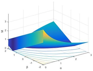
We define $M$ is the sum of absolute value of $\left(\mathbf{K}{\mathbf{x}}_{\alpha ,\beta }^{\delta }-{\mathbf{y}}^{\delta }\right)$. When $\delta =$ 0.01 and $n=$ 60, using the ergodic searching treatment to find the relationship between $M$ and the combinations of regularization parameters ($\alpha$, $\beta$), the most suitable value of parameters ($\alpha$, $\beta$) can be found. The results are shown in Fig. 1. When $\delta =$ 0.1 and $n=$ 60, the results are shown in Fig. 2.

Fig. 1Relationship between M and (α, β) with small perturbation δ= 0.01

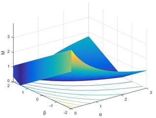
Fig. 2Relationship between M and (α, β) with big perturbation δ= 0.1

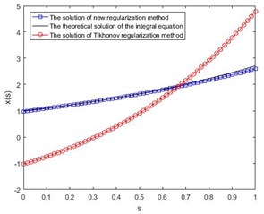
When $\delta =$ 0.01 and $n=$ 60, the theoretical solution of Eq. (3) and the solutions of different regularization methods are shown in Fig. 3. While $\delta =$ 0.1 and $n=$ 60, the results are shown in Fig. 4. It can be seen from Figs. 3 and 4 that the new regularization method proposed in this article presents much better results than those by conventional Tikhonov method for both small and big perturbations, which shows the validity and stability of the new method.

Fig. 3Comparison of numerical results with small perturbation δ= 0.01

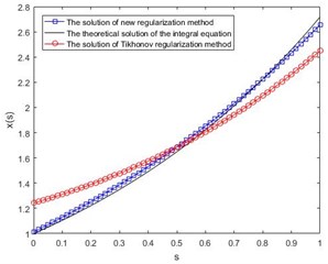
Fig. 4Comparison of numerical results with big perturbation δ= 0.1

5. Conclusions

To improve the solution accuracy of ill-posed problems, in this paper we propose a new regularization method and prove its rationality from the view of mathematics. Furthermore, we demonstrate the convergence of its solution and present a selection method of the regularization parameters when using the new regularization method. Numerical tests have been made for solving the first kind Fredholm integral equation and comparing the results with the classical Tikhonov regularization method. Numerical results show that the present method can provide much better approximation of true solution, especially in the case of the ill-posed problems with big perturbation. Because of regularization methods are applied to obtain the solution of ill-conditioned inverse problems by solving a family of neighboring well-posed problems, if we want to get good numerical results, the error in practical engineering of measuring progress requires high, otherwise will enlarge the final result of the error, the new regularization method which reduces the need for measurement errors. A disadvantage of the new regularization method is the ergodic searching of its regularization parameters, which needs huge computational cost and should be further optimized in the coming research.

References

-
Tikhonov A. N., Arsenin Yl. V. A Solution of Ill-Posed Problems. Wiley, New York, 1977.
Landweber L. An iteration formula for Fredholm integral equations of the first kind. Journal of Mathematics, Vol. 73, Issue 3, 1951, p. 615-624.
Linjun Wang, Xun Han, Jie Liu A new regularization method and application to dynamic load identification problems. Inverse Problems in Science and Engineering, Vol. 19, Issue 6, 2011, p. 765-776.
Dym C. L., Lang M. A. A modified tikhonov regularization method for solving ill-posed problems – (1) construction of regularization. Chinese Quarterly Journal of Mathematics, Vol. 15, Issue 2, 2000, p. 98-101.
Billel Neggal, Nadjib Boussetila, Faouzia Rebbani Projected Tikhonov regularization method for Fredholm integral equations of the first kind. Journal of Inequalities and Applications, Vol. 1, 2016, p. 2016-195.
Hansen P. C. Analysis of discrete ill-posed problems by means of the L-curve. Siam Review, Vol. 34, Issue 4, 1992, p. 561-580.
Calvetti D. Tikhonov regularization and the L-curve for large discrete ill-posed problems. Journal of Computational and Applied Mathematics, Vol. 123, Issues 1-2, 2000, p. 423-446.
Cited by
About this article
This work is supported by the strategic Priority Research Program of the Chinese Academy of Sciences, Grant No. XDB22040502.