The influence of the smoothing component on the quality of algebraic forecasts

1. Introduction

Time series forecasting is important area in many fields of science, engineering and finance. Time series forecasting aim is to build model from previously observed values and to use it to predict future values. Conditionally, these methods can be classified into long-term, medium and short-term time series forecasting techniques [1]. The class of short-term forecasting techniques include models with a short future horizons. A one-step forward future horizon is adequate for short-term time series forecasting [1] delivering methods which are widely used in finance [3-5]; electricity price/load, solar and wind energy forecasting problem [6, 7]; passenger demand [8] and many others.

Many publications of short term time series forecasting concentrates on practical applications of classical linear and statistical methods for day-ahead forecasting. Simplest of them are moving average and simple exponential smoothing [9], Holt-Winters methods [10] or Autoregressive Integrated Moving Average type models (ARIMA, ARMAX, ARMAX, SARIMA etc.) [11, 12]. In spite of numerous amount of forecasting models and techniques, there cannot be a universal forecasting model that could be applied for all situations.

An algebraic prediction techniques based on the identification of the skeleton algebraic sequences in short-term time series is developed in [13-15]. The main objective of this paper is to analyze error components and internal smoothing influence to mixed smoothing forecasting model of an algebraic interpolant [15]. Since the main purpose of this model is to remove noise term from time series and to identify algebraic sequence, it is very important to calibrate well suited object function. The goal is to develop such a predictor which could produce reliable forecasts for short time series under investigation.

This paper is organized as follows. Algebraic prediction with mixed smoothing is discussed in Section 2; computational experiments are discussed in Section 3 and concluding remarks are given in the last section.

2. Algebraic model with mixed smoothing

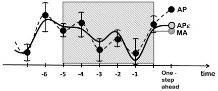
The algebraic time series forecasting model with smoothing procedure has been introduced in [14, 15]. The main idea of the smoothing procedure is based on conciliation between the variability of the algebraic interpolant and the smoothness of moving average time series estimates – instead of trying to make a straight forward projection of this algebraic model into the future. There is made an assumption that real world time series observations $\left\{x_k\right\}$, $k=$ 0, 1, …, 2$n$ are contaminated with an additive noise $\left\{{\epsilon }_k\right\}$, $k=$ 0, 1, …, 2$n$. Skeleton algebraic sequence can be identified by removing this noise: ${\tilde{x}}_k=x_k-{\epsilon }_k$, $k=$ 0, 1, …, 2$n$.

Fig. 1A schematic diagram illustrating the algebraic time series forecasting method by cancelling noise from original observations: thick dots denote the original time series, solid line denotes the corrected time series, AP – algebraic forecasting for original time series; APε – algebraic forecasting for the corrected time series; MA – forecasting using smoothing method for the corrected time series

The objective function is constructed in order to compress this noise [15]:

where ${\stackrel{-}{x}}_{2n+1}$ is a smoothing component for the one step ahead future value; ${\widehat{x}}_{2n+1}$ algebraic prediction using recurrent linear sequences presented in [13-15] when sequence order is $n$; $E$ is the error computed between the observations $\left\{{\tilde{x}}_k\right\}$, $k=$ 0, 1, …, 2$n$ and the reconstructed algebraic skeleton $\left\{{\widehat{x}}_k\right\}$, $k=$ 0, 1, …, 2$n$. Parameters $a$ and $b$ are penalty proportions between different terms in the denominator of the fitness function. Evolutionary algorithms are used to find near optimal sequence of corrections [13-15].

In this study we determine the influence of the error term $E$ and preferred smoothing model on the forecasting accuracy.

3. Computational experiments

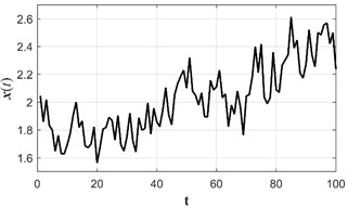
All computations use electricity supply in Euro area (EA11-2000, EA12-2006, EA13-2007, EA15-2008, EA16-2010, EA17-2013, EA18-2014, EA19) time series (2008-01-01 to 2016-04-31 monthly data by Gigawatts per hour) [16]. Data scale in Fig. 2 is divided by 10000. The model builds on the initial 21 observations. The accuracy of the predictions is computed using RMSE metrics. The order of the algebraic model in this case is determined to be $n=$ 4.

Fig. 2Electricity supply in Euro area (EA11-2000, EA12-2006, EA13-2007, EA15-2008, EA16-2010, EA17-2013, EA18-2014, EA19) time series where monthly data are observed from 2008-01-01 to 2016-04-31

3.1. A dependence of the forecasting accuracy on components of the target function

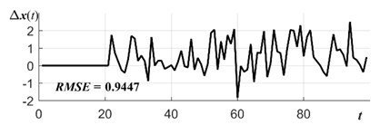
Let us consider object function case where$a=b=$ 0. In this case Algebraic forecasting model does not involve error metrics and smoothing factor into the optimization process. External smoothing is performed by averaging 100 reconstructed algebraic skeletons for every single prediction instead. Root mean square error (RMSE) is computed for predicted values. Forecasting errors is presented in Fig. 3(a) where RMSE = 0.9447.

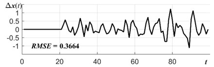
Now consider object function case where $a=$ 1 and $b=$ 0. Forecasting errors are sufficiently reduced when Error component is involved into optimization procedure. Now the results are obtained without using any smoothing. Forecasting errors is presented in Fig. 3(b) where RMSE = 0.3664.

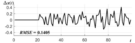
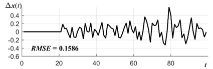
Even better prediction results are obtained when a smoothing parameter is used in the object function (the case where $a=$ 0 and $b=$ 1). Smoothing component there is moving average forecasting at $s=$ 2 – MA(2). As we can see in Fig. 3(c), the forecasting errors of such model are lowest RMSE = 0.1405. Mixed algebraic prediction model (where $a=b=$ 1) does not outperform these results: Fig. 3(d) RMSE = 0.1586.

Fig. 3Electrical supply time series forecasting errors for: a) algebraic prediction (AP) with external smoothing (a=b= 0), b) AP with error component (a= 1, b= 0), c) AP with internal smoothing (a=0, b= 1), d) AP with mixed smoothing a=b= 1

a)

b)

c)

d)

3.2. A dependence of the forecasting accuracy on components of the target function

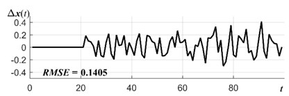
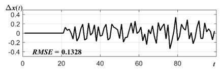
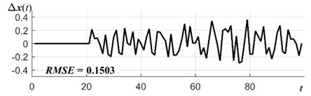
We continue computational experiments with electrical supply time series and compare the functionality of the Algebraic prediction with different smoothing models. We consider object function case where $a=$ 0 and $b=$ 1. Moving average (MA), simple exponential smoothing (SES) and ARIMA models are tested on electrical supply time series. The best smoothing models are obtained when MA parameter is $s=$ 2, SES parameter is $\alpha =0.85$ and ARIMA(1,1,0). Forecasting errors are presented in Fig. 4. It is clear that algebraic time series forecasting with internal smoothing SES(0.85) outperforms MA(2) and ARIMA(1,1,0). RMES value for SES(0.85) is 0.1328, for MA(2) is 0.1405 and for ARIMA(1,1,0) is 0.1503. As we can see from previous section forecasting results are better with any smoothing model than results without smoothing.

Fig. 4Algebraic time series forecasting errors with internal smoothing model is: a) MA(2), b) SES(0.85), c) ARIMA(1,1,0)

a)

b)

c)

4. Conclusions

Algebraic time series forecasting model is analyzed in this study. The influence of the smoothing and error parameters in considered. Computational experiments with electrical supply time series show that smoothing component in the object function has the strongest influence on the time series forecasting results. Different smoothing models in the object function produced different accuracy of the predictions. Algebraic forecasting results with any internal smoothing model outperformed results of the forecasting without smoothing. Error parameter in the object function does not have such significant influence on forecasting results, but still helps to reduce forecasting errors.