Variable learning rate EASI-based adaptive blind source separation in situation of nonstationary source and linear time-varying systems

2.1. Description of adaptive BSS

In traditional BSS, the mixing matrix $\mathbf{A}$ is constant. However, in reality, the way in which signals mix varies with time. We call the linear instantaneous mixing matrix ${\mathbf{A}}_t$. The model can be described as [25, 27, 28]:

where $\mathbf{X}\left(t\right)=\left[{\overrightarrow{x}}_1\right(t),{\overrightarrow{x}}_2(t),...,{\overrightarrow{x}}_m(t){]}^T\in R^{m\times L}$ denotes the observed signals, ${\mathbf{A}}_t\in R^{m\times k}$, and $\mathbf{N}\left(t\right)\in R^{m\times L}$ denotes the observation noise. $\mathbf{S}\left(t\right)=\left[{\overrightarrow{s}}_1\right(t),{\overrightarrow{s}}_2(t),...,{\overrightarrow{s}}_k(t){]}^T\in R^{k\times L}$ represents the nonstationary source signals. Without considering any observation noise:

In our setting, the separation matrix ${\mathbf{B}}_t\in R^{k\times m}$ is unknown but should vary with time, and the separated multiple nonstationary independent signals $\mathit{Y}\left(t\right)=\left[{\overrightarrow{y}}_1\right(t),{\overrightarrow{y}}_2(t),...,{\overrightarrow{y}}_k(t){]}^T\in R^{k\times L}$ can be got by:

and the separated signals latest value $\overrightarrow{y}\left(t\right)={\mathbf{B}}_t\overrightarrow{x}\left(t\right)={\mathbf{B}}_t{\mathbf{A}}_t\overrightarrow{s}\left(t\right)={\mathbf{E}}_t\overrightarrow{s}\left(t\right)\in R^{k\times 1}$. We hope that the $\mathbf{Y}\left(\mathit{t}\right)$ and $\mathbf{S}\left(t\right)$ are as similar as possible. Fig. 1 illustrates the adaptive BSS model for linear instantaneous mixing systems and nonstationary source signals.

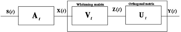
The separating matrix ${\mathbf{B}}_t$ is constructed using either a one-stage or two-stage separation system [16, 29]. In the one-stage method, ${\mathbf{B}}_t$ is obtained directly by minimizing/maximizing some contrast function. In this paper, we focus on the two-stage approach, in which the observations are first preprocessed by an $m$×$m$ whitening matrix ${\mathbf{V}}_t$, and then an orthogonal matrix ${\mathbf{U}}_t\in R^{k\times m}$ is used to separate the source signals. Finally, we obtain the total separating matrix ${\mathbf{B}}_t={\mathbf{U}}_t{\mathbf{V}}_t$. Fig. 2 illustrates this process.

Fig. 1Adaptive BSS model for linear instantaneous time-varying mixing systems and nonstationary source signals

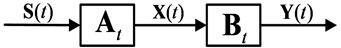
Fig. 2Two-stage separation adaptive BSS

2.2. Model assumptions of adaptive BSS

BSS problems have multiple solutions [28]. To identify the optimal solution, five basic assumptions are proposed, which are slightly different from those used in traditional BSS [14]:

1) ${\mathbf{A}}_t\in R^{m\times k}$ satisfies $rank\left({\mathbf{A}}_t\right)=k$.

2) $\overrightarrow{s}\left(t\right)$ is a nonstationary random process.

3) $\overrightarrow{s}\left(t\right)$ is statistically independent at each time, and at most one component in $\mathbf{S}\left(t\right)$ obeys a Gaussian distribution.

4) The number of observed signals $\mathbf{X}\left(t\right)$ is greater than or equal to the number of source signals $\mathbf{S}\left(t\right)$.

5) $\mathbf{S}\left(t\right)$ is linearly mixed and the system is slowly time-varying.

2.3. Comparison of adaptive BSS and traditional BSS

Table 1 summarizes the differences between adaptive BSS and traditional BSS in terms of the source signals and mixing matrix.

3.1. Notion of equivariance

The EASI algorithm was first proposed by Cardoso, who used the notion of equivariance to prove that the performance of EASI is independent of the mixing matrix [29] when the mixing matrix is constant. In the same way, a blind estimate of ${\mathbf{A}}_t$ is simply a function of $\mathbf{X}\left(t\right)$. This can be expressed as:

where ${\widehat{\mathbf{A}}}_t$ is the estimator of ${\mathbf{A}}_t$ and $\mathbf{F}(\cdot )$ represents this functional relationship. In equivariance theory, when the data conversion is equivalent to some parameter conversion, both ${\widehat{\mathbf{A}}}_t$ and $\mathbf{X}\left(t\right)$ are multiplied on the left by a matrix $\mathbf{M}\in R^{k\times k}$. In this case, ${\widehat{\mathbf{A}}}_t$ is equivariant when it satisfies:

Eq. (6) shows that $\widehat{\mathbf{S}}\left(t\right)$ is given by $\widehat{\mathbf{S}}\left(t\right)=\mathbf{F}\left(\mathbf{S}\right(t\left){)}^{-1}\mathbf{S}\right(t)$, which means that it is only related to $\mathbf{S}\left(t\right)$ and is independent of ${\mathbf{A}}_t$: this is also called uniform performance.

3.2. Serial matrix updating

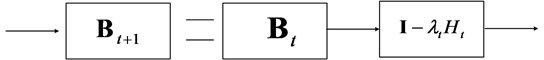
The core concept of EASI is serial updating [16]. Serial updating involves choosing a $k$×$k$ matrix-valued function $y\to H\left(y\right)$, which is used to update the separating matrix ${\mathbf{B}}_{t+1}$ according to:

where ${\lambda }_t$ is the learning rate and is fixed in traditional EASI algorithm. Fig. 3 illustrates this update process of separation matrix. The global system ${\mathbf{E}}_{t+1}$ can be similarly updated by:

Eq. (8) also shows that the overall system ${\mathbf{E}}_t$ is not dependent on ${\mathbf{A}}_t$.

Fig. 3Serial update of a matrix

3.3. EASI algorithm

Using the notion of ‘relative gradient’ [16], the function $H\left(y\right)$ in Eq. (7) can be considered as:

In Eq. (9), $f$ is an arbitrary differentiable function. Therefore, ${\mathbf{B}}_{t+1}$ can be updated according to:

Let $\mathbf{I}\in R^{k\times k}$ be the unit matrix. Exactly as in Eq. (10), according to [16], the serial whitening matrix ${\mathbf{V}}_{t+1}$ can be updated by:

where $\overrightarrow{y}\left(t\right)={\mathbf{U}}_t\overrightarrow{z}\left(t\right)$ and $\overrightarrow{z}\left(t\right)={\mathbf{V}}_t\overrightarrow{x}\left(t\right)$ is the signal after whitening. The orthogonal matrix ${\mathbf{U}}_{t+1}$ can also be updated by:

The purpose of Eq. (11) and Eq. (12) is to obtain the updated ${\mathbf{B}}_{t+1}$. Then, according to Eq. (11), Eq. (12), and ${\mathbf{B}}_t={\mathbf{U}}_t{\mathbf{V}}_t$, we have:

In this equation, $E\left(f\mathrm{\text{'}}\right(\overrightarrow{y}\left(t\right)\left){\overrightarrow{y}}^T\right(t)-\overrightarrow{y}(t\left)f\mathrm{\text{'}}\right(\overrightarrow{y}\left(t\right){)}^T+\overrightarrow{y}\left(t\right){\overrightarrow{y}}^T\left(t\right)-\mathbf{I})=$ 0, and so for $i\ne j$, $\overrightarrow{y}\left(i\right)$ and $\overrightarrow{y}\left(j\right)$ are independent of each other. For $k$ arbitrary nonlinear functions $g\left(y\right)$, we define:

The EASI algorithm for adaptive source separation is based on Eq. (7) and Eq. (15):

To maintain uniform performance, which means that ${\mathbf{B}}_t$ can take any values, we adjust $H\left(\overrightarrow{y}\right(t\left)\right)$ to preserve stability. Eq. (17) describes the normalized form [16]:

3.4. Advantages of EASI algorithm

EASI is a gradient-based algorithm that uses nonlinear decorrelation to estimate the independent components. It has several advantages over other ICA algorithms [30].

1) EASI is an adaptive and online algorithm, which makes it suitable for problems in which the underlying distributions of input characteristics vary over time.

2) EASI is equivariant, and the convergence speeds, interference suppression levels, and other properties are only related to the signals’ normalized distributions and are independent of the mixing matrix.

3) EASI offers improved parallelism by combining whitening with separation, because other methods whiten the input features during a preprocessing step.

4) EASI is computationally efficient, as its basic operations only require addition and multiplication.

3.5. Variable learning rate EASI algorithm

In the EASI algorithm, the learning rate is closely related to the convergence speed and steady-state error. When the learning rate is fixed, values that are too large will make the algorithm unstable, whereas values that are too small will increase the convergence time [17].

Given the limitations of a fixed learning rate, we use a typical time-descending learning rate given by [31, 32]:

where ${\lambda }_0$, $t_0$, and $t_d$ are constants.

3.6. Scope and conditions of variable learning rate EASI algorithm

1) The sources are statistically independent.

2) The source signals are non-stationary and the mixing matrix represents slow instantaneous linear mixing.

3) The number of observed signals is greater than or equal to the number of source signals, and the number of signals cannot be changed.

4.1. Simulation dataset and parameter settings

We design simulations to demonstrate the performance of our variable learning rate EASI-based adaptive BSS method. We choose three different signals, a nonstationary wave ${\overrightarrow{s}}_1\left(t\right)$, square wave ${\overrightarrow{s}}_2\left(t\right)$, and a triangular wave ${\overrightarrow{s}}_3\left(t\right)$. These are specified as follows:

${\overrightarrow{s}}_1\left(t\right)$, ${\overrightarrow{s}}_2\left(t\right)$, and ${\overrightarrow{s}}_3\left(t\right)$ are independent of each other. For ${\overrightarrow{s}}_1\left(t\right)$, which is not periodic, we calculate the expectation at intervals [1, 400 s] and [201, 600 s] to be 0.0118 and 0.0082 and the mean square root to be 1.4982 and 1.0013, respectively. The expectation and mean square root change with time. Therefore, ${\overrightarrow{s}}_1\left(t\right)$ has the property of non-stationarity. The linear instantaneous mixing matrix ${\mathbf{A}}_t\in R^{3\times 3}$ is slowly time-varying. We use MATLAB’s “rand” function to randomly generate ${\mathbf{A}}_t$ as follows:

Then, we allow the first element of ${\mathbf{A}}_t$ to vary slowly:

Therefore, we have designed nonstationary sources and a slowly time-varying mixing matrix. The nonlinear functions $\overrightarrow{g}\left(\overrightarrow{y}\right(t\left)\right)$ are related to the signal distributions. When $\overrightarrow{y}\left(t\right)$ is a sup-Gaussian signal, the choice may be $\overrightarrow{g}\left(\overrightarrow{y}\right(t\left)\right)=\overrightarrow{y}(t{)}^3$. When $\overrightarrow{y}\left(t\right)$ is a super-Gaussian signal, our choice is usually $\overrightarrow{g}\left(\overrightarrow{y}\right(t\left)\right)=\mathrm{t}\mathrm{a}\mathrm{n}\mathrm{h}\left(\overrightarrow{y}\right(t\left)\right)$ [17]. In this paper, $\overrightarrow{g}\left(\overrightarrow{y}\right(t\left)\right)=\overrightarrow{y}(t{)}^3$. The sampling length $L=$ 2000 s.

For comparison, we designed a fixed learning rate EASI, RLS method, and variable learning rate EASI. For the fixed learning rate algorithm, after a lot of experiments, we set the EASI learning rate to 0.0017 and the RLS learning rate to 0.982. For the variable learning rate parameters, we set ${\lambda }_0=$ 0.014, $t_0=$ 200, and $t_d=$ 0.025.

4.2. Source separation evaluation index

4.3. Simulation results

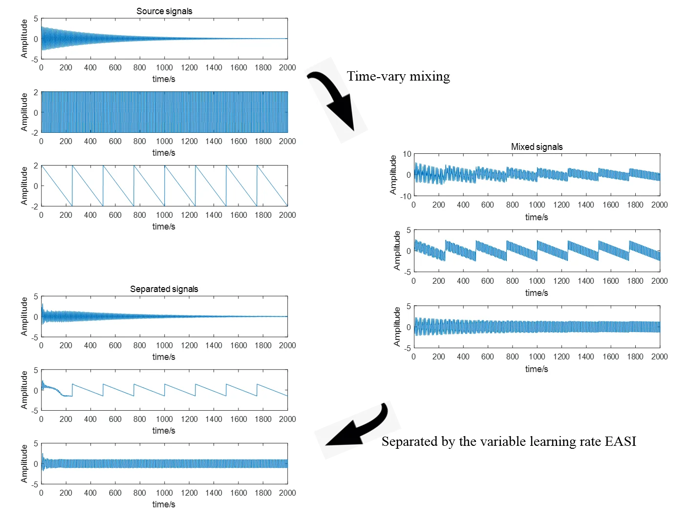
The source signals used in this simulation are shown in Fig. 4. From top to bottom, they are a non-stationary wave ${\overrightarrow{s}}_1\left(t\right)$, a square wave ${\overrightarrow{s}}_2\left(t\right)$, and a triangular wave ${\overrightarrow{s}}_3\left(t\right)$. After linear instantaneous mixing, the observed signals are shown in Fig. 5. Figs. 6-9 show the separation results of the fixed learning rate EASI, the fixed learning rate RLS, and the variable learning rate EASI method.

Fig. 4Three different nonstationary source signals

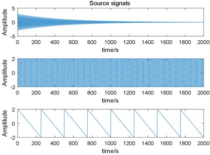
Fig. 5Signals after linear mixing

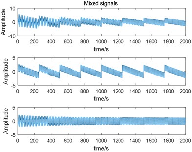
Fig. 6Estimated signals output by the fixed learning rate EASI algorithm

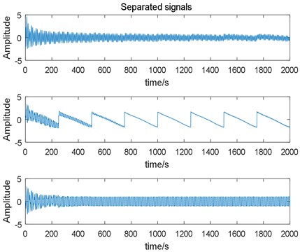
Fig. 7Estimated signals output by the fixed learning rate RLS algorithm

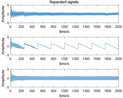
Fig. 8Estimated signals output by the variable learning rate EASI algorithm

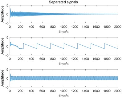
Table 2 presents the separation results achieved by EASI, RLS, and variable learning rate EASI. Table 3 demonstrates the independence of the source signals. Table 4 lists the similarity between the separated signals given by EASI, RLS, and variable learning rate EASI.

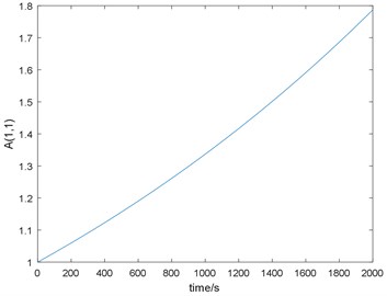
Fig. 9 shows the variation of the first element of the mixing matrix over time.

Fig. 9The variation of A1(1,1)

4.4. Simulation results analysis

The simulation results can be analyzed as follows:

1) The first separation signal in Fig. 6 corresponds to the first source signal in Fig. 4, the second separation signal ${\overrightarrow{y}}_2\left(t\right)$ corresponds to the third source signal ${\overrightarrow{s}}_3\left(t\right)$, and ${\overrightarrow{y}}_3\left(t\right)$ corresponds to ${\overrightarrow{s}}_2\left(t\right)$. The sequence of the separated signals is uncertain, which is a problem with the adaptive BSS algorithm.

2) From Fig. 4, we can see that ${\overrightarrow{s}}_1\left(t\right)$ is nonstationary. In Table 3, if the $p$-value is close to 0, the source signals are not independent. Therefore, the sources are nonstationary and independent, and can be used to verity the algorithm.

3) The shapes of the identified signals are similar to those of the source signals (see Fig. 4 and Figs. 6-8) in the different methods. This result is confirmed by Table 2. The fixed learning rate EASI and RLS are not as good as variable learning rate EASI in the case of nonstationary environments and time-varying mixing.

4) In Table 4, the similarity coefficient between separated signals is less than 6 % in variable learning rate EASI, demonstrating that the correlation between the separated signals is not high and the separation is very good.

5) Fig. 9 illustrates the exponential increase of ${\mathbf{A}}_1\left(\mathrm{1,1}\right)$. Though ${\mathbf{A}}_1$ was chosen at random, the selection of the initial value ${\mathbf{A}}_1\left(\mathrm{1,1}\right)$ has a significant influence on the simulation results. The reason for this requires further study.

6) In Tables 2 and 4, the variable learning rate has a significant impact on the results. The variable learning rate EASI achieves better results than the other algorithms, and RLS outperforms EASI. The separation signals obtained by all methods are similar to the source signals, and the correlation between the separated signals is not high.

7) Similarity coefficients and VQM can both be used to evaluate the separation results. In Table 2, when the similarity coefficients are the same, VQM can still distinguish the results.