Nonlinear mechanical system simulation based on modal coordinates and modal forces

1. Introduction

There are many ways to calculate the forced response to a linear mechanical system. Some of those methods, such as calculating the response as a convolution between the input force and the impulse response, are computation intensive. The author therefore introduced a way to use digital filters to calculate the response in a paper 2003, [1]. The method was well suited to include nonlinearities attached to the linear system. That unique method was described for instance in a paper 2006, [2]. The calculations were fast, but a bias error was introduced. The bias error was identified for the digital filter method and related ones as Runge-Kutta and State Space. The results were described in several papers, such as [3].

The digital filter functions for nonlinear systems were collected in a nonlinear MATLAB toolbox, which have been used in many companies and universities. It was presented at an IMAC conference 2007, [4].

In the toolbox, the functions could handle systems with many nonlinearities, but only one input force could be treated. There was a need to be able to simulate many simultaneous input forces, so a method, building on modal coordinates and modal forces, has been developed.

2. Linear system

For a linear mechanical system, the transfer function $H_{ij}$ between a force input in point $j$ and a displacement response in point $i$ may be written as:

where $R_{ij}$ are the residues and $s_m$ are the poles. $*$ stands for complex conjugate. For each $m$, we can get $R_{ij}$ by:

where $r$ is a reference point. Care has to be taken when selecting $r$, so that all modes are excited. The sign of the square roots has to be carefully selected as well. $R_i$ and $R_j$ corresponds to scaled mode shapes.

With many input forces, we can now calculate the modal forces, one for each mode, by multiplying with the corresponding $R_j$:

where $F$ is a matrix with the applied forces in columns. With $N$ as the numbers of time samples, $NF$ the number of forces, and $Nm$ as the number of modes:

We now apply each modal force to the corresponding function:

We do that with a digital filter, using ramp invariant method and MATLAB function filter. The filter coefficients are determined by:

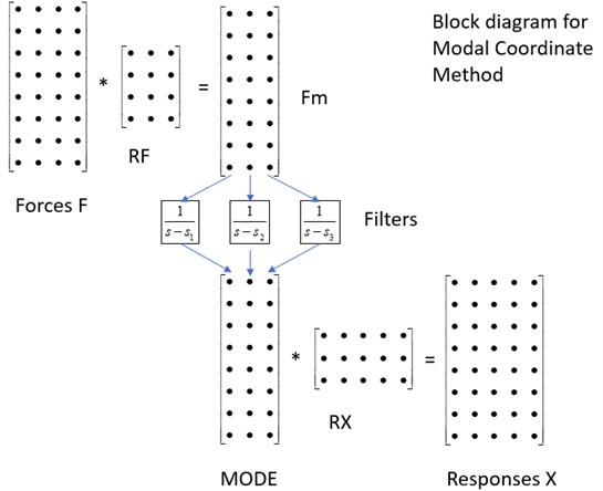
where $T$ is the time step, inverse of sampling frequency. After filtering, the modes may be combined to displacement and/or velocity at selected outputs by multiplying with corresponding factors, similar to Eq. (3). As we are only using half of Eq. (1), to get the result we have to take 2 times the real part. Fig. 1. shows the principle.

Fig. 1Block diagram for modal coordinate method

A function timerespdv using the method above has the syntax:

The linear system is defined by mass matrix $M$, damping matrix $C$ and stiffness matrix $K$. The applied forces are given as time histories with sampling frequency $fs$ in columns of $F$. The degree of freedom numbers, DOFS, for reference, applied forces and wanted responses are given. mods is a vector telling which modes to use, numbered in frequency order.

A version where the linear system is defined by residues and poles is also made:

3. Linear system with nonlinearities

The method above may be extended to a linear system with localized nonlinear elements added at certain DOFs. The nonlinear forces should be zero memory, which means they may be expressed as functions of displacement and/or velocity at DOFs where they are attached.

The filtering in the process is taken one time step at a time. For mode m, the value at sample $n$ may be written as:

where NLFM is the modal nonlinear force, calculated the same way as the modal applied force. A big part of this, $Q_m$, may be calculated from what is already known:

so:

which should be fulfilled for all modes. An estimate of the modes gives estimates of displacement and velocities at DOFs where there are nonlinearities. The nonlinear functions are explicitly given in the code, so the modal force NLFM can be calculated. This gives a new estimate of the modes. The procedure goes on until convergence. A typical number of needed iterations is five to six.

Here are some examples of nonlinear functions in the MATLAB code.

A cubic spring at one DOF, ND(1), to ground and a gap with end stiffness between another DOF, ND(2), and ground:

if abs(ND(2)) < 0.0001

nlf = 0;

else

nlf = 1000*(ND(2)-sign(ND(2))*0.0001);

end

NFD = [0.2e7*ND(1).^3, nlf];

and a “square with sign damper” using velocity at DOF NV(1):

4. Example

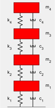
A four degree of freedom system, fourdof, is used, Fig. 2.

Two nonlinear elements are added, a cubic spring between DOF 4 and ground, and a “square with sign damper” from DOF 3 to ground. Two random forces are applied, one to DOF 4 and one to DOF 2. All four displacement responses and all four velocity responses are calculated.

Fig. 2Four degree of freedom linear system

Part of the test script:

RDOF = 4;FDOFS = [2 4];NDD = 4;NVD = 3;

XDOFS = 1:4;VDOFS = 1:4;

mods = 1:4;

F = [F2 F4];

[X,V] = nonlin_mck_modal_c(F,fs,M,C,K,RDOF,FDOFS,NDD,NVD,XDOFS,VDOFS,mods).

To validate, the nonlinear forces are calculated from the responses, and those are applied to the linear system together with the two applied forces:

FD = 1.7e15*X(:,4).^3;

FV = 2.e6*V(:,3).*abs(V(:,3));

FDOFS = [2 3 4];

[XX,VV] = timerespdv([F2 -FV F4-FD],fs,M,C,K,RDOF,FDOFS,XDOFS,VDOFS,mods).

Comparison:

$\frac{norm\left(X-XX\right)}{norm\left(XX\right)},\frac{norm\left(V-VV\right)}{norm\left(VV\right)}.$

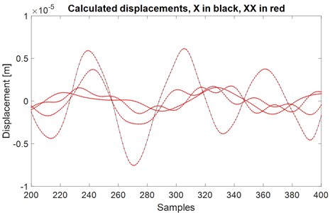
Result typically around 10^-5.

A plot of part of $X$ and $XX$ is shown in Fig. 3.

Fig. 3Comparison of calculated displacements for validation

References

-
Ahlin K. On the use of digital filters for mechanical system simulation. Proceedings of 74th Shock and Vibration Symposium, San Diego, 2003.
Ahlin K., Magnevall M., Josefsson A. Simulation of forced response in linear and nonlinear mechanical systems using digital filters. International Conference on Noise and Vibration Engineering, Leuven, 2006.
Chen Y., Ahlin K., Linderholt A. Bias errors for different methods of simulating linear and nonlinear systems. Proceedings of the 33rd IMAC, A Conference and Exposition on Structural Dynamics, 2015.
Ahlin K., Brandt A., Lagö T. A new MATLAB toolbox for simulation and parameter identification of nonlinear mechanical systems. IMAC-XXV: A Conference and Exposition on Structural Dynamics, Orlando, Florida, USA, 2007.
About this article