An explicit closed-form solution for transverse and longitudinal vibration of beam with multi-directional elastic constraints under an arbitrary moving load

Ding, Yong; Han, Lingxia; You, Jiuang

doi:10.21595/jve.2019.20172

Journal of Vibroengineering

Browse Journal

Submit article

Published: 15 November 2019

Check for updates

An explicit closed-form solution for transverse and longitudinal vibration of beam with multi-directional elastic constraints under an arbitrary moving load

Yong Ding¹

Lingxia Han²

Jiuang You³

^{1, 2, 3}Department of Civil Engineering, Ningbo University, Ningbo, China

Corresponding Author:

Yong Ding

Cite the article Download PDF

Downloads 1430

Abstract

Beams with elastic constraints are widely used in dynamic systems in engineering. A general explicit solution is presented here for the vibration of simple span beam with transverse, rotational and axial elastic boundary constraints due to an arbitrary moving load. The Euler-Bernoulli beam theory is adopted, in which the boundary constraints are treated as multi-directional boundary springs. After the modal analyses, the explicit closed-form solutions of transverse and axial vibration of the beam under a constant, sinusoidal and cosinoidal moving loads are obtained, respectively. And the vibration of a beam subjected to an arbitrary moving load is derived by the superposition of Fourier series. The current analytical solution is exact and can be applied in multiple engineering fields to obtain accurate structural vibrations. In numerical examples, the effects of the boundary springs on the natural frequencies, modes, deflection, bending moment and boundary reaction of the beam are studied in details. The effects of the number of terms in Fourier series of arbitrary moving load are also discussed.

An explicit closed-form solution for transverse and longitudinal vibration of beam with multi-directional elastic constraints under an arbitrary moving load

Highlights

A closed-form explicit solution for the transverse and axial vibrations of the beam with transverse, rotational and axial boundary springs subjected to a moving load.
The analytical solution is exact and can be applied in multiple engineering fields to obtain accurate structural vibrations.
The proposed solution is consistent with FEM result, and can be applied to verify the FEM analysis.
Effect of the parameters, such as boundary spring coefficients and moving-load velocity, on the dynamic response is provided.

1. Introduction

Dynamic analysis of the beam due to moving load is an important research topic in engineering, which is widely applied in bridges, railways, mechanical process, micro-structures, piping systems, etc., [1-3]. Many studies have been performed to explore the various aspects of this moving load problem [1], and most of them are concerned with the transverse vibration of the beam. The early work on the behavior of a beam subjected to a constant moving load was reported by Timoshenko [4]. Fryba [5] studied the vibration of a simply supported beam subject to a moving load using Laplace-Carson integral transformation technology. Hilal et al. [6, 7] investigated the vibration of a single span beam with hinged or fixed boundary conditions using the Duhamel’s integral technology, in which a constant or harmonic load traveling on the beam with accelerating, decelerating and constant velocity, respectively. Yang et al. [8] studied the vibration of the cracked inhomogeneous cantilever beam under a fixed axial force and a moving transverse load. Ouyang and Wang [9] explored the effect of the axially moving forces on the transverse vibration of the rotating beam. Şimşek et al. [10] analyzed the dynamics of elastically supported functionally graded beam systems, in which the displacement of the beam is assumed as a sum of power functions and the equations of motion are derived using the Hamilton’s principle. In the work of Zhu and Law [11], the vibration of multi-span continuous beam is analyzed, and the moving load is identified.

There are not so many studies on the longitudinal vibration of the beam subjected to moving load. Dmitriev [12] presented the early analytical solution on the longitudinal vibration of the beam subjected to a constant axial force and fixed axially in one end. Mamandi et al. [13] studied analytically not only the transverse vibration, but also the longitudinal vibration of inclined beam subjected to a moving load. The effects of the transverse or axial elastic constraint on the longitudinal vibration were also considered in the researches of Nguyen and Duhamel [14], Wu [15], Toth and Ruge [16], but the means adopted in their works are the finite element method, not the analytical solution.

Considering that the analytical solution is exact and can be applied in multiple engineering fields to obtain accurate structural vibration or to validate the numerical analysis, a general analytical solution is presented in this paper for the transverse and longitudinal vibration of beam subjected to an arbitrary moving load. Differs from the previous research, it is an explicit closed-form solution, and the multi-directional boundary springs are considered to cope with the elastic boundary constraints widely adopted in engineering [2, 16, 17]. The Euler-Bernoulli beam theory is adopted. The eigensolutions for the transverse and longitudinal vibration are deduced firstly in modal analysis. Then the explicit closed-form solution is presented for the forced vibration of the beam under a constant, sinusoidal and cosinoidal moving load respectively with a constant velocity through modal superposition method. And then the vibration of a beam subjected to an arbitrary moving load is obtained by the technology of Fourier expansion. Finally, the effects of the different elastic boundary spring and number of Fourier series of the arbitrary moving load on the vibration of the beam are discussed.

2. Theory and formulations

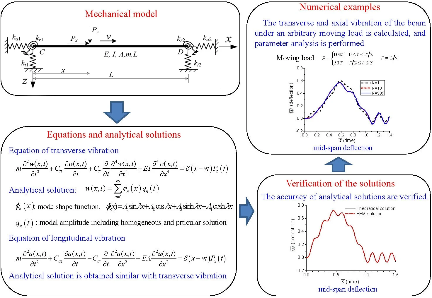
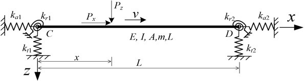
A single span Euler-Bernoulli beam with multi-directional boundary springs is shown in Fig. 1, in which $k_{a i}$ , $k_{r i}$ and $k_{t i}$ ( $i =$ 1, 2) are the constants of axial, rotational and transverse springs, respectively. These boundary springs represent the multi-directional elastic boundary in engineering structures, such as bridge [3, 11] and functionally graded beam [10]. $P_{x}$ , $P_{z}$ are axial and transverse load respectively moving with a constant velocity of $v$ . $E$ , $I$ , $A$ , $m$ and $L$ are Young’s modulus of material, the moment of inertia of cross-section, the area, the mass per unit length and the length of the beam, respectively. The transverse and longitudinal vibrations of the beam are analyzed independently, and the nonlinear effect is neglected in the current work.

Fig. 1A single span with multi-directional elastic boundary springs under moving loads

2.1. Transverse vibration

The transverse vibration is governed by the following partial differential equation:

1a

m \frac{\partial^{2} w (x, t)}{\partial t^{2}} + C_{t e} \frac{\partial w (x, t)}{\partial t} + C_{t i} \frac{\partial}{\partial t} \frac{\partial^{4} w (x, t)}{\partial x^{4}} + E I \frac{\partial^{4} w (x, t)}{\partial x^{4}} = δ (x - v t) P_{z} (t),

where $δ (\cdot)$ is Dirac delta function; $C_{t e}$ and $C_{t i}$ are the external and internal damping coefficients, respectively. If the Rayleigh damping is adopted, they are proportional to the mass and stiffness of the beam, respectively:

1b

C_{t e} = α_{t} m, C_{t i} = β_{t} E I,

where $α_{t}$ and $β_{t}$ are proportional constants. The transverse displacement, $w (x, t)$ , is written in modal form:

2

w (x, t) = \sum_{n = 1}^{\infty} ϕ_{n} (x) q_{n} (t),

where $ϕ_{n} (x)$ is mode shape function from modal analysis, and $q_{n} (t)$ is the modal amplitude from forced vibration analysis. Substituting Eq. (2) into Eq. (1), and multiplying by $ϕ_{n} (x)$ , integrating with respect to $x$ from 0 to $L$ , and applying the orthogonal conditions, the equations about the modal amplitude is obtained:

3

{\ddot{q}}_{n} (t) + 2 ζ_{t, n} ω_{n} {\dot{q}}_{n} (t) + ω_{n}^{2} q_{n} (t) = \frac{ϕ_{n} (v t) P_{z} (t)}{M_{t, n}}, n = 1,2, \dots, \infty,

where $ζ_{t, n}$ , $ω_{n}$ and $M_{t, n}$ are the modal damping ratio, modal frequency and modal mass for the $n$ th mode, respectively, and:

4

M_{t, n} = \int_{0}^{L} ϕ_{n}^{2} (x) m d x .

The damping ratio from the Rayleigh damping is:

5

ζ_{t, n} = \frac{α_{t} + β_{t} ω_{n}^{2}}{2 ω_{n}} .

2.1.1. Modal analysis of transverse vibration

The associated eigenvalue problem of the beam in transverse vibration is [18]:

6a

ϕ'''' (x) - λ^{4} ϕ (x) = 0,

where:

6b

λ^{4} = \frac{ω^{2} m}{E I} .

In which $ω$ is the circular frequency. The boundary conditions of the beam with the boundary springs shown in Fig. 1 are:

7

\begin{array}{l} k_{t 1} ϕ (0) = - E I ϕ^{'''} (0), \\ - E I ϕ^{''} (0) = - k_{r 1} ϕ^{'} (0), \\ k_{t 2} ϕ (L) = E I ϕ^{'''} (L), \\ - E I ϕ^{''} (L) = k_{r 2} ϕ^{'} (L) . \end{array}

The general solution of Eq. 6(a) is:

8

ϕ (x) = A_{1} s i n λ x + A_{2} c o s λ x + A_{3} s i n h λ x + A_{4} c o s h λ x .

Substituting Eq. (8) into Eqs. (7), the equations of the constants of $A_{i}$ ( $i =$ 1, 2, 3, 4) are derived as:

9

K_{t} A_{t} = [\begin{array}{l} K_{11} & K_{12} & K_{13} & K_{14} \\ K_{21} & K_{22} & K_{23} & K_{24} \\ K_{31} & K_{32} & K_{33} & K_{34} \\ K_{41} & K_{42} & K_{43} & K_{44} \end{array}] \{\begin{array}{l} A_{1} \\ A_{2} \\ A_{3} \\ A_{4} \end{array}\} = \{\begin{array}{l} 0 \\ 0 \\ 0 \\ 0 \end{array}\} .

The elements of the matrix $K_{t}$ are:

10

\begin{array}{l} K_{11} = - K_{13} = - E I λ^{3}, K_{12} = K_{14} = k_{t 1}, K_{21} = K_{23} = k_{r 1}, K_{22} = - K_{24} = E I λ, \\ K_{31} = k_{t 2} s i n λ L + E I λ^{3} c o s λ L, K_{32} = k_{t 2} c o s λ L - E I λ^{3} s i n λ L, \\ K_{33} = k_{t 2} s i n h λ L - E I λ^{3} c o s h λ L, K_{34} = k_{t 2} c o s h λ L - E I λ^{3} s i n h λ L, \\ K_{41} = E I λ^{2} s i n λ L - k_{r 2} λ c o s λ L, K_{42} = E I λ^{2} c o s λ L + k_{r 2} λ s i n λ L, \\ K_{43} = - E I λ^{2} s i n h λ L - k_{r 2} λ c o s h λ L, K_{44} = - E I λ^{2} c o s h λ L - k_{r 2} λ s i n h λ L, \end{array}

thus, the characteristic equation of this system is obtained from the existence of the non-trivial solutions of Eq. (9) and expressed as:

11

d e t (K_{t}) = 0 .

The eigenvalues, $λ_{n}$ ( $n = 1,2, . . ., \infty$ ), are obtained from Eq. (11). Then the eigenfunctions, $ϕ_{n} (x)$ , are deduced from Eq. (9), in which the constants of the $n$ th mode are $A_{1, n} =$ 1:

12

A_{2, n} = \frac{K_{33} (K_{44} K_{21} - K_{24} K_{41}) + K_{34} (K_{41} K_{23} - K_{43} K_{21}) + K_{31} (K_{43} K_{24} - K_{44} K_{23})}{K_{24} (K_{42} K_{33} - K_{43} K_{32}) + K_{34} (K_{43} K_{22} - K_{42} K_{23}) + K_{44} (K_{32} K_{23} - K_{22} K_{33})},

A_{3, n} = \frac{K_{22} (K_{44} K_{31} - K_{34} K_{41}) + K_{42} (K_{34} K_{21} - K_{31} K_{24}) + K_{32} (K_{24} K_{41} - K_{44} K_{21})}{K_{24} (K_{42} K_{33} - K_{43} K_{32}) + K_{34} (K_{43} K_{22} - K_{42} K_{23}) + K_{44} (K_{32} K_{23} - K_{22} K_{33})},

A_{4, n} = \frac{K_{21} (K_{43} K_{32} - K_{42} K_{33}) + K_{31} (K_{42} K_{23} - K_{43} K_{22}) + K_{41} (K_{22} K_{33} - K_{32} K_{23})}{K_{24} (K_{42} K_{33} - K_{43} K_{32}) + K_{34} (K_{43} K_{22} - K_{42} K_{23}) + K_{44} (K_{32} K_{23} - K_{22} K_{33})},

n = 1,2, . . ., \infty .

2.1.2. Forced vibration analysis of transverse vibration

Although the modal amplitude in forced vibration, $q_{n} (t)$ , can be solved numerically by Duhamel’s integral technology, an analytical solution is more clear and helpful to understand the behavior of vibration [6, 7]. To consider an arbitrary moving load, $P_{z} (t)$ in Eq. (3) is expressed as Fourier series firstly:

13

P_{z} (t) = \frac{a_{0}}{2} + \sum_{n = 1}^{\infty} [a_{n} c o s \frac{2 n π (t - T)}{T} + b_{n} s i n \frac{2 n π (t - T)}{T}], n = 1, . . ., \infty,

where $T$ is the time while the moving load is on the beam, $T = L / v$ :

14

a_{n} = \frac{2}{T} \int_{0}^{T} P_{z} (t) c o s \frac{2 n π (t - T)}{T} d t, b_{n} = \frac{2}{T} \int_{0}^{T} P_{z} (t) s i n \frac{2 n π (t - T)}{T} d t,

If the solutions of Eq. (3) for constant, sinusoidal and cosinoidal moving loads are derived respectively, the general analytical solution for an arbitrary moving load can be obtained by the superposition of a series of solutions.

When the moving load is a constant, $P_{z} (t) = P_{z 0}$ , the solution of Eq. (3) is:

15

q_{n} (t) = q_{n}^{'} (t) + q_{n}^{''} (t),

where $q_{n}^{'} (t)$ and $q_{n}^{''} (t)$ are the homogeneous and the particular solutions, respectively. The particular solution is assumed as:

16

q_{n}^{''} (t) = B_{1, n} s i n λ_{n} v t + B_{2, n} c o s λ_{n} v t + B_{3, n} s i n h λ_{n} v t + B_{4, n} c o s h λ_{n} v t .

Substituting Eq. (16) into Eq. (3) and considering the equation is valid at any time, the multipliers of $s i n λ_{n} v t$ , $c o s λ_{n} v t$ , $s i n h λ_{n} v t$ and $c o s h λ_{n} v t$ are equal to zero, respectively. So that the constants in Eq. (16) are derived as:

17

\begin{array}{l} B_{1, n} = \frac{[(ω_{n}^{2} - λ_{n}^{2} v^{2}) + 2 A_{2, n} ζ_{t, n} ω_{n} λ_{n} v] P_{z 0}}{[{(ω_{n}^{2} - λ_{n}^{2} v^{2})}^{2} + {(2 ζ_{t, n} ω_{n} λ_{n} v)}^{2}] M_{t, n}}, \\ B_{2, n} = \frac{[- 2 ζ_{t, n} ω_{n} λ_{n} v + A_{2, n} (ω_{n}^{2} - λ_{n}^{2} v^{2})] P_{z 0}}{[{(ω_{n}^{2} - λ_{n}^{2} v^{2})}^{2} + {(2 ζ_{t, n} ω_{n} λ_{n} v)}^{2}] M_{t, n}}, \\ B_{3, n} = \frac{[A_{3, n} (ω_{n}^{2} + λ_{n}^{2} v^{2}) - 2 A_{4, n} ζ_{t, n} ω_{n} λ_{n} v] P_{z 0}}{[{(ω_{n}^{2} + λ_{n}^{2} v^{2})}^{2} - {(2 ζ_{t, n} ω_{n} λ_{n} v)}^{2}] M_{t, n}}, \\ B_{4, n} = \frac{[2 A_{3, n} ζ_{t, n} ω_{n} λ_{n} v - A_{4, n} (ω_{n}^{2} + λ_{n}^{2} v^{2})] P_{z 0}}{[- {(ω_{n}^{2} + λ_{n}^{2} v^{2})}^{2} + {(2 ζ_{t, n} ω_{n} λ_{n} v)}^{2}] M_{t, n}}, n = 1, . . ., \infty . \end{array}

The homogeneous solution is:

18

q_{n}^{'} (t) = e^{- ζ_{t, n} ω_{n} t} (D_{1, n} c o s ω_{D, n} t + D_{2, n} s i n ω_{D, n} t),

where $ω_{D, n}$ is the natural frequency considering the damping ratio:

19

ω_{D, n} = ω_{n} \sqrt{1 - ζ_{t, n}^{2}} .

The constants $D_{1, n}$ and $D_{2, n}$ are determined by imposing the initial conditions of Eq. (20) and obtained in Eq. (21):

20

q_{n} (0) = 0, {\dot{q}}_{n} (0) = 0,

21

D_{1, n} = - B_{2, n} - B_{4, n}, D_{2, n} = - \frac{(B_{1, n} λ_{n} v + B_{2, n} ζ_{n} ω_{n} + B_{3, n} λ_{n} v + B_{4, n} ζ_{n} ω_{n})}{ω_{D n}},

when the moving load is an sinusoidal function, $P_{z} (t) = P_{z 0} s i n (Ω t + φ)$ , the solution of Eq. (3) is still as Eq. (15). The particular solution is assumed as:

22

\begin{array}{l} {q''}_{n} (t) = {B'}_{1, n} c o s [(λ_{n} v + Ω) t + φ] + {B'}_{2, n} c o s [(λ_{n} v - Ω) t - φ] \\ + {B'}_{3, n} s i n [(λ_{n} v + Ω) t + φ] + {B'}_{4, n} s i n [(λ_{n} v - Ω) t - φ] + {B'}_{5, n} e^{λ_{n} v t} c o s (Ω t + φ) \\ + {B'}_{6, n} e^{- λ_{n} v t} c o s (Ω t + φ) + {B'}_{7, n} e^{λ_{n} v t} s i n (Ω t + φ) + {B'}_{8, n} e^{- λ_{n} v t} s i n (Ω t + φ) . \end{array}

Substituting Eq. (22) into Eq. (3) and considering the equation is valid at any time, the multipliers of $c o s [(λ_{n} v + Ω) t + φ],$ $c o s [(λ_{n} v - Ω) t - φ],$ $s i n [(λ_{n} v + Ω) t + φ],$ $s i n [(λ_{n} v - Ω) t - φ],$ $e^{λ_{n} v t} c o s (Ω t + φ),$ $e^{- λ_{n} v t} c o s (Ω t + φ),$ $e^{λ_{n} v t} s i n (Ω t + φ),$ $e^{- λ_{n} v t} s i n (Ω t + φ)$ are equal to zero, respectively. So that the constants in Eq. (22) are derived as:

23

{B^{'}}_{1, n} = - \frac{s_{0} (A_{1, n} s_{1} + A_{2, n} s_{2})}{s_{1}^{2} + s_{2}^{2}}, {B^{'}}_{2, n} = \frac{s_{0} (A_{1, n} s_{3} + A_{2, n} s_{4})}{s_{3}^{2} + s_{4}^{2}},

{B^{'}}_{3, n} = \frac{s_{0} (A_{2, n} s_{1} - A_{1, n} s_{2})}{s_{1}^{2} + s_{2}^{2}}, {B^{'}}_{4, n} = \frac{s_{0} (- A_{2, n} s_{3} + A_{1, n} s_{4})}{s_{3}^{2} + s_{4}^{2}},

{B^{'}}_{5, n} = - \frac{s_{0} s_{5} (A_{3, n} + A_{4, n})}{s_{5}^{2} + s_{6}^{2}}, {B^{'}}_{6, n} = \frac{s_{0} s_{7} (- A_{3, n} + A_{4, n})}{s_{7}^{2} + s_{8}^{2}},

{B^{'}}_{7, n} = \frac{s_{0} s_{6} (A_{3, n} + A_{4, n})}{s_{5}^{2} + s_{6}^{2}}, {B^{'}}_{8, n} = \frac{s_{0} s_{8} (- A_{3, n} + A_{4, n})}{s_{7}^{2} + s_{8}^{2}},

s_{0} = \frac{P_{0}}{2 M_{t, n}}, s_{1} = ω_{n}^{2} - {(λ_{n} v + Ω)}^{2}, s_{2} = 2 ζ_{t, n} ω_{n} (λ_{n} v + Ω),

s_{3} = ω_{n}^{2} - {(λ_{n} v - Ω)}^{2}, s_{4} = 2 ζ_{t, n} ω_{n} (λ_{n} v - Ω), s_{5} = 2 Ω (λ_{n} v + ζ_{t, n} ω_{n}),

s_{6} = {(λ_{n} v)}^{2} - Ω^{2} + 2 ζ_{t, n} ω_{n} λ_{n} v + ω_{n}^{2}, s_{7} = 2 Ω (λ_{n} v - ζ_{t, n} ω_{n}),

s_{8} = {(λ_{n} v)}^{2} - Ω^{2} - 2 ζ_{t, n} ω_{n} λ_{n} v + ω_{n}^{2}, n = 1, . . ., \infty .

The homogeneous solution is:

24

{q^{'}}_{n} (t) = e^{- ζ_{t, n} ω_{n} t} ({D^{'}}_{1, n} c o s ω_{D n} t + {D^{'}}_{2, n} s i n ω_{D n} t),

where the constants ${D'}_{1, n}$ and ${D'}_{2, n}$ are determined by imposing the initial conditions of Eq. (20) and obtained in Eq. (25):

25

{D^{'}}_{1, n} = - ({B^{'}}_{1, n} + {B^{'}}_{2, n} + {B^{'}}_{5, n} + {B^{'}}_{6, n}) c o s φ - ({B^{'}}_{3, n} - {B^{'}}_{4, n} + {B^{'}}_{7, n} + {B^{'}}_{8, n}) s i n φ,

\begin{array}{l} {D'}_{2, n} = - [- {B'}_{1, n} (λ_{n} v + Ω) s i n φ + {B'}_{2, n} (λ_{n} v - Ω) s i n φ + {B'}_{3, n} (λ_{n} v + Ω) c o s φ \\ + {B'}_{4, n} (λ_{n} v - Ω) c o s φ + {B'}_{5, n} (λ_{n} v c o s φ - Ω s i n φ) - {B'}_{6, n} (λ_{n} v c o s φ + Ω s i n φ) \\ + {B'}_{7, n} (λ_{n} v s i n φ + Ω c o s φ) - {B'}_{8, n} (λ_{n} v s i n φ - Ω c o s φ) - ζ_{t, n} ω_{n} {D'}_{1, n}] / ω_{D, n}, \end{array}

when the moving load is an cosinoidal function, $P_{z} (t) = P_{z 0} c o s (Ω t + φ)$ , the solution of Eq. (3) is still as Eq. (15). The particular solution is assumed as:

26

\begin{array}{l} {q''}_{n} (t) = {B''}_{1, n} c o s [(λ_{n} v + Ω) t + φ] + {B''}_{2, n} c o s [(λ_{n} v - Ω) t - φ] \\ + {B''}_{3, n} s i n [(λ_{n} v + Ω) t + φ] + {B''}_{4, n} s i n [(λ_{n} v - Ω) t - φ] + {B''}_{5, n} e^{λ_{n} v t} c o s (Ω t + φ) \\ + {B''}_{6, n} e^{- λ_{n} v t} c o s (Ω t + φ) + {B''}_{7, n} e^{λ_{n} v t} s i n (Ω t + φ) + {B''}_{8, n} e^{- λ_{n} v t} s i n (Ω t + φ) . \end{array}

Substituting Eq. (26) into Eq. (3) and considering the equation is valid at any time, the multipliers of $c o s [(λ_{n} v + Ω) t + φ],$ $c o s [(λ_{n} v - Ω) t - φ],$ $s i n [(λ_{n} v + Ω) t + φ],$ $s i n [(λ_{n} v - Ω) t - φ],$ $e^{λ_{n} v t} c o s (Ω t + φ),$ $e^{- λ_{n} v t} c o s (Ω t + φ),$ $e^{λ_{n} v t} s i n (Ω t + φ),$ $e^{- λ_{n} v t} s i n (Ω t + φ)$ are equal to zero, respectively. So that the constants in Eq. (26) are derived as:

27

{B^{''}}_{1, n} = \frac{s_{0} (A_{2, n} s_{1} - A_{1, n} s_{2})}{s_{1}^{2} + s_{2}^{2}}, {B^{''}}_{2, n} = \frac{s_{0} (A_{2, n} s_{3} - A_{1, n} s_{4})}{s_{3}^{2} + s_{4}^{2}},

{B''}_{3, n} = \frac{s_{0} (A_{1, n} s_{1} + A_{2, n} s_{2})}{s_{1}^{2} + s_{2}^{2}}, {B''}_{4, n} = \frac{s_{0} (A_{1, n} s_{3} + A_{2, n} s_{4})}{s_{3}^{2} + s_{4}^{2}},

{B^{''}}_{5, n} = \frac{s_{0} s_{6} (A_{3, n} + A_{4, n})}{s_{5}^{2} + s_{6}^{2}}, {B^{''}}_{6, n} = \frac{s_{0} s_{8} (- A_{3, n} + A_{4, n})}{s_{7}^{2} + s_{8}^{2}},

{B''}_{7, n} = \frac{s_{0} s_{5} (A_{3, n} + A_{4, n})}{s_{5}^{2} + s_{6}^{2}}, {B''}_{8, n} = \frac{s_{0} s_{7} (A_{3, n} - A_{4, n})}{s_{7}^{2} + s_{8}^{2}}, n = 1, . . ., \infty,

where the expression of $s_{i}$ ( $i =$ 0, 1, ..., 8) is same as that in Eq. (23).

The homogeneous solution is:

28

q_{n}^{'} (t) = e^{- ζ_{t, n} ω_{n} t} ({D^{''}}_{1, n} c o s ω_{D, n} t + {D^{''}}_{2, n} s i n ω_{D, n} t),

where the constants ${D''}_{1, n}$ and ${D''}_{2, n}$ are determined by imposing the initial conditions of Eq. (20) and obtained in Eq. (29):

29

{D''}_{1, n} = - ({B''}_{1, n} + {B''}_{2, n} + {B''}_{5, n} + {B''}_{6, n}) c o s φ - ({B''}_{3, n} - {B''}_{4, n} + {B''}_{7, n} + {B''}_{8, n}) s i n φ,

\begin{array}{l} {D''}_{2, n} = - [- {B''}_{1, n} (λ_{n} v + Ω) s i n φ + {B''}_{2, n} (λ_{n} v - Ω) s i n φ + {B''}_{3, n} (λ_{n} v + Ω) c o s φ \\ + {B''}_{4, n} (λ_{n} v - Ω) c o s φ + {B''}_{5, n} (λ_{n} v c o s φ - Ω s i n φ) - {B''}_{6, n} (λ_{n} v c o s φ + Ω s i n φ) \\ + {B''}_{7, n} (λ_{n} v s i n φ + Ω c o s φ) - {B''}_{8, n} (λ_{n} v s i n φ - Ω c o s φ) - ζ_{t, n} ω_{n} {D''}_{1, n}] / ω_{D, n} . \end{array}

After the general solution of transverse vibration is obtained, the bending moment of the beam could be derived:

30

M (x, t) = - E I \frac{\partial^{2} w (x, t)}{\partial x^{2}} .

2.2. Longitudinal vibration

The longitudinal vibration is governed by the following partial differential equation:

31

m \frac{\partial^{2} u (x, t)}{\partial t^{2}} + C_{a e} \frac{\partial u (x, t)}{\partial t} - C_{a i} \frac{\partial}{\partial t} \frac{\partial^{2} u (x, t)}{\partial x^{2}} - E A \frac{\partial^{2} u (x, t)}{\partial x^{2}} = δ (x - v t) P_{x} (t),

where $C_{a e}$ and $C_{a i}$ are the external and internal damping coefficients in longitudinal vibration, respectively. If the Rayleigh damping is adopted:

32

C_{a e} = α_{a} m, C_{a i} = β_{a} E A,

where $α_{a}$ and $β_{a}$ are proportional constant. The longitudinal displacement is expressed as:

33

w (x, t) = \sum_{n = 1}^{\infty} ψ_{n} (x) r_{n} (t),

where $ψ_{n} (x)$ is the mode shape function, and $r_{n} (t)$ is the modal amplitude. Similar to Eq. (3) in transverse vibration, the equation of modal amplitude in longitudinal vibration is:

34

{\ddot{r}}_{n} (t) + 2 ζ_{a, n} ω_{n} {\dot{r}}_{n} (t) + ω_{n}^{2} r_{n} (t) = \frac{ψ_{n} (v t) P_{x} (t)}{M_{a, n}}, n = 1,2, \dots, \infty,

where $ζ_{a, n}$ and $M_{a, n}$ are the modal damping ratio and modal mass in longitudinal vibration, respectively, and:

35

M_{a, n} = \int_{0}^{L} m ψ_{n}^{2} (x) d x .

The damping ratio from the Rayleigh damping is:

36

ζ_{a, n} = \frac{α_{a} + β_{a} ω_{n}^{2}}{2 ω_{n}} .

The mode shape and amplitude are also derived from modal and forced vibration analysis, receptively.

2.2.1. Modal analysis of longitudinal vibration

Following the general procedure of deduction [18], the associated eigenvalue problem in longitudinal vibration of the beam in Fig. 1 is:

37a

ψ'' (x) + e^{2} ψ (x) = 0,

where:

37b

e^{2} = \frac{ω^{2} m}{E A} .

The axial boundary conditions are:

38a

k_{a 1} ψ (0) = E A ψ^{'} (0),

38b

k_{a 2} ψ (L) = - E A ψ^{'} (L) .

Considering the existence of the non-trivial solutions, the equation of eigenvalue is:

39

(E^{2} A^{2} e^{2} - k_{a 1} k_{a 2}) s i n e L - (k_{a 1} + k_{a 2}) E A e c o s e L = 0 .

The eigenvalues, $e_{n}$ ( $n =$ 1, 2, ..., $\infty$ ), are derived from Eq. (39). Then the eigenfunctions, $ψ_{n} (x)$ , are obtained:

40

ψ_{n} (x) = c o s e_{n} x + \frac{k_{a 1}}{E A e_{n}} s i n e_{n} x, n = 1,2, . . ., \infty .

2.2.2. Forced vibration analysis of longitudinal vibration

The modal amplitude, $r_{n} (t)$ , in Eq. (34) is solved analytically in this section. The arbitrary axial moving load, $P_{x} (t)$ , can also be expressed as Fourier series similar to the transverse load, $P_{z} (t)$ , in Eq. (13). After the modal amplitudes of vibration of the beam under constant, sinusoidal and cosinoidal longitudinal moving loads are derived respectively, that under an arbitrary moving load can be obtained using the method of superposition.

When the moving load keeps a constant, $P_{x} (t) = P_{x 0}$ , the solution of Eq. (34) is:

41

r_{n} (t) = r_{n}^{'} (t) + r_{n}^{''} (t),

where $r_{n}^{'} (t)$ and $r_{n}^{''} (t)$ are the homogeneous and particular solutions, respectively.

The particular solution is assumed as:

42

{r^{''}}_{n} (t) = C_{1, n} c o s e_{n} v t + C_{2, n} s i n e_{n} v t .

Substituting Eq. (42) into Eq. (34) and considering the equation is valid at any time, the multipliers of $c o s e_{n} v t$ and $s i n e_{n} v t$ are equal to zero, respectively. So that the constants in Eq. (42) are derived as:

43

C_{1, n} = \frac{P_{x 0} [E A e_{n} (ω_{n}^{2} - e_{n}^{2} v^{2}) - 2 k_{a 1} ζ_{a, n} ω_{n} e_{n} v]}{M_{a, n} E A e_{n} [{(ω_{n}^{2} - e_{n}^{2} v^{2})}^{2} + {(2 ζ_{a, n} ω_{n} e_{n} v)}^{2}]},

C_{2, n} = \frac{P_{x 0} [k_{a 1} (ω_{n}^{2} - e_{n}^{2} v^{2}) + 2 ζ_{a, n} ω_{n} e_{n} v E A e_{n}]}{M_{a, n} E A e_{n} [{(ω_{n}^{2} - e_{n}^{2} v^{2})}^{2} + {(2 ζ_{a, n} ω_{n} e_{n} v)}^{2}]}, n = 1, . . ., \infty .

The homogeneous solution is:

44

{r^{'}}_{n} (t) = e^{- ζ_{a, n} ω_{n} t} (E_{1, n} c o s ω_{D, n} t + E_{2, n} s i n ω_{D, n} t) .

The constants $E_{1, n}$ and $E_{2, n}$ are determined by imposing the initial conditions of Eq. (45) and obtained in Eq. (46):

45

r_{n} (0) = 0, {\dot{r}}_{n} (0) = 0,

46

E_{1, n} = - C_{1, n}, E_{2, n} = - \frac{(C_{1, n} ζ_{a, n} ω_{n} + C_{2, n} e_{n} v)}{ω_{D, n},}

when the moving load is an sinusoidal function, $P_{x} (t) = P_{x 0} s i n (Ω t + φ)$ , the solution of Eq. (34) is still as Eq. (41), where the particular solution is assumed as:

47

\begin{array}{l} {r''}_{n} (t) = {C'}_{1, n} c o s [(e_{n} v + Ω) t + φ] + {C'}_{2, n} c o s [(e_{n} v - Ω) t - φ] \\ + {C'}_{3, n} s i n [(e_{n} v + Ω) t + φ] + {C'}_{4, n} s i n [(e_{n} v - Ω) t - φ] . \end{array}

Substituting Eq. (47) into Eq. (34) and considering the equation is valid at any time, the multipliers of $c o s [(e_{n} v + Ω) t + φ],$ $c o s [(e_{n} v - Ω) t - φ],$ $s i n [(e_{n} v + Ω) t + φ],$ $s i n [(e_{n} v - Ω) t - φ]$ are equal to zero, respectively. So that the constants in Eq. (47) are derived as:

48

{C^{'}}_{1, n} = - \frac{d_{0} \{C_{s} d_{1} + d_{2}\}}{d_{1}^{2} + d_{2}^{3}}, {C^{'}}_{2, n} = \frac{d_{0} \{C_{s} d_{3} + d_{4}\}}{d_{3}^{2} + d_{4}^{2}}, {C^{'}}_{3, n} = \frac{d_{0} [d_{1} - d_{2} C_{s}]}{d_{1}^{2} + d_{2}^{2}},

{C^{'}}_{4, n} = \frac{d_{0} \{- d_{3} + C_{s} d_{4}\}}{d_{3}^{2} + d_{4}^{2}}, d_{0} = \frac{P_{x 0}}{2 M_{a, n}}, d_{1} = ω_{n}^{2} - {(e_{n} v + Ω)}^{2},

d_{2} = 2 ζ_{a, n} ω_{n} (e_{n} v + Ω), d_{3} = ω_{n}^{2} - {(e_{n} v - Ω)}^{2},

d_{4} = 2 ζ_{a, n} ω_{n} (e_{n} v - Ω), C_{s} = \frac{k_{a 1}}{E A e_{n}}, n = 1, . . ., \infty .

The homogeneous solution is:

49

{r^{'}}_{n} (t) = e^{- ζ_{a, n} ω_{n} t} ({E^{'}}_{1, n} c o s ω_{D, n} t + {E^{'}}_{2, n} s i n ω_{D, n} t),

where the constants ${E'}_{1, n}$ and ${E'}_{2, n}$ are determined by imposing the initial conditions of Eq. (45) and obtained in Eq. (50):

50

{E^{'}}_{1, n} = - ({C^{'}}_{1, n} + {C^{'}}_{2, n}) c o s φ - ({C^{'}}_{3, n} - {C^{'}}_{4, n}) s i n φ,

\begin{array}{l} {E'}_{2, n} = - [- {C'}_{1, n} (e_{n} v + Ω) s i n φ + {C'}_{2, n} (e_{n} v - Ω) s i n φ + {C'}_{3, n} (e_{n} v + Ω) c o s φ \\ + {C'}_{4, n} (e_{n} v - Ω) c o s φ - ζ_{a, n} ω_{n} {E'}_{1, n}] / ω_{D n}, \end{array}

when the moving load is an cosinoidal function, $P_{x} (t) = P_{x 0} c o s (Ω t + φ)$ , the solution of Eq. (34) is still as Eq. (41). The particular solution is assumed as:

51

{r^{''}}_{n} (t) = {C^{''}}_{1, n} c o s [(e_{n} v + Ω) t + φ] + {C^{''}}_{2, n} c o s [(e_{n} v - Ω) t - φ]

+ {C''}_{3, n} s i n [(e_{n} v + Ω) t + φ] + {C''}_{4, n} s i n [(e_{n} v - Ω) t - φ] .

Substituting Eq. (51) into Eq. (34) and considering the equation is valid at any time, the multipliers of $c o s [(e_{n} v + Ω) t + φ],$ $c o s [(e_{n} v - Ω) t - φ],$ $s i n [(e_{n} v + Ω) t + φ],$ $s i n [(e_{n} v - Ω) t - φ]$ are equal to zero, respectively. So that the constants in Eq. (51) are derived as:

52

{C^{''}}_{1, n} = \frac{d_{0} \{d_{1} - d_{2} C_{s}\}}{d_{1}^{2} + d_{2}^{3}}, {C^{''}}_{2, n} = \frac{d_{0} \{d_{3} - d_{4} C_{s}\}}{d_{3}^{2} + d_{4}^{2}}, {C^{''}}_{3, n} = \frac{d_{0} [d_{1} C_{s} + d_{2}]}{d_{1}^{2} + d_{2}^{2}},

{C''}_{4, n} = \frac{d_{0} \{d_{3} C_{s} + d_{4}\}}{d_{3}^{2} + d_{4}^{2}}, n = 1, . . ., \infty,

where the expressions of $d_{i}$ ( $i =$ 0, ..., 4) and $C_{s}$ are same as Eq. (48). The homogeneous solution is:

53

{q^{'}}_{n} (t) = e^{- ζ_{a, n} ω_{n} t} ({E^{''}}_{1, n} c o s ω_{D, n} t + {E^{''}}_{2, n} s i n ω_{D, n} t),

where the constants ${E''}_{1, n}$ and ${E''}_{2, n}$ are determined by imposing the initial conditions of Eq. (45) and obtained in Eq. (54):

54

{E^{''}}_{1, n} = - ({C^{''}}_{1, n} + {C^{''}}_{2, n}) c o s φ - ({C^{''}}_{3, n} - {C^{''}}_{4, n}) s i n φ,

\begin{array}{l} {E''}_{2, n} = - [- {C''}_{1, n} (e_{n} v + Ω) s i n φ + {C''}_{2, n} (e_{n} v - Ω) s i n φ + {C''}_{3, n} (e_{n} v + Ω) c o s φ \\ + {C''}_{4, n} (e_{n} v - Ω) c o s φ - ζ_{a, n} ω_{n} {E''}_{1, n}] / ω_{D, n} . \end{array}

After the displacement in longitudinal vibration is obtained, the axial force is derived:

55

N (x, t) = E A \frac{\partial u (x, t)}{\partial x} .

3. Numerical results and discussion

To clarify the analysis, ten examples (EP) are presented, where the properties of the beam, boundary springs and moving loads are shown in Tables 1, 2. The beam properties in Table 1 are taken from the properties of typical beam in hinged-jointed slab bridge [3]. The constants of transverse springs in Table 2, $k_{t 1}$ and $k_{t 2}$ , are calculated from the rubber bearing in bridge engineering. If the area of the rubber bearing is 0.01 m², height is 0.06 m and elastic modulus is 360 MPa, the constant of the transverse spring is 0.6×10⁸ N/m. The constants of rotational springs, $k_{r 1}$ and $k_{r 2}$ , are derived from simple-span bridges with continuous deck [3]. The constants of axial springs, $k_{a 1}$ and $k_{a 2}$ , are similar with those of transverse springs. The loads used in Table 2 are constant moving load and varying moving load.

Some results from the current analytical solutions are compared with those from finite element method (FEM) analyses. The effects of boundary springs on the vibration of the beam under moving load are studied. And the number of terms used in the Fourier series of arbitrary load is discussed.

Table 1Beam properties

$I$	0.0655 m⁴	$L$	19.3 m
$E$	34.5 GPa	$m$	1770 kg/m
$A$	1 m²	$ζ_{t, n}$ , $ζ_{a, n}$	0.005

3.1. Comparison between analytical solutions and FEM analyses

In this section, the results from analytical solutions are compared with those from FEM analyses. In analytical solution, modal and dynamic analyses of the beam in Table 1, 2 are performed by using the method in Section 2. In FEM analysis, the beam is divided into 80 Euler-Bernoulli beam elements, the modes and natural frequencies of free vibration are calculated by solving the characteristic equation with the subspace iteration method, and the dynamic response of the beam under moving load are obtained by using modal superposition method [17, 19, 20].

Table 2Properties of boundary springs and moving loads in numerical examples

No.	$k_{t 1}$ (N/m)	$k_{t 2}$ (N/m)	$k_{r 1}$ (N⋅m)	$k_{r 2}$ (N⋅m)	$k_{a 1}$ (N/m)	$k_{a 2}$ (N/m)	Load (N)
1	∞	∞	0	0	∞	0	$P_{z} = 100 δ (x - v t)$ , $P_{x} = 0$
2	1.2×10⁸	1.2×10⁸	0	0	∞	0	$P_{z} = 100 δ (x - v t)$ , $P_{x} = 0$
3	0.6×10⁸	0.6×10⁸	0	0	∞	0	$P_{z} = 100 δ (x - v t)$ , $P_{x} = 0$
4	∞	∞	1.7×10⁸	1.7×10⁸	∞	0	$P_{z} = 100 δ (x - v t)$ , $P_{x} = 0$
5	∞	∞	3.4×10⁸	3.4×10⁸	∞	0	$P_{z} = 100 δ (x - v t)$ , $P_{x} = 0$
6	∞	∞	0	0	∞	0	$P_{z} = 0$ , $P_{x} = 100 δ (x - v t)$
7	∞	∞	0	0	1.5×10⁷	0	$P_{z} = 0$ , $P_{x} = 100 δ (x - v t)$
8	∞	∞	0	0	1.5×10⁶	0	$P_{z} = 0$ , $P_{x} = 100 δ (x - v t)$
9	1.2×10⁸	1.2×10⁸	0	0	∞	0	$P_{z} = \{\begin{array}{l} 100 t δ (x - v t), \\ 50 T δ (x - v t), \end{array} \begin{array}{l} 0 \leq t < T / 2 \\ T / 2 \leq t \leq T \end{array}$ $T = L / v$ , $P_{x} = 0$
10	∞	∞	0	0	1.5×10⁷	0	$P_{x} = \{\begin{array}{l} 100 t δ (x - v t), \\ 50 T δ (x - v t), \end{array} \begin{array}{l} 0 \leq t < T / 2 \\ T / 2 \leq t \leq T \end{array}$ $T = L / v$ , $P_{z} = 0$

In modal analysis, the first four modes and natural frequencies of the beam in Examples 1-8 are calculated and shown in Table 3. The results from the analytical solutions are nearly identical with those from the FEM analyses.

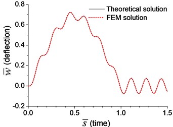
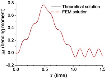
In dynamic analysis, the moving-load-induced mid-span deflection and bending moment of the beam with transverse springs in Example 3 and with rotational springs in Example 4 are calculated, and the results are shown in Fig. 2 and Fig. 3, respectively. The velocity of the moving load is assumed as $0.1 v_{c r}$ , where $v_{c r}$ is the critical velocity [5]:

56

v_{c r} = 2 f_{1} L .

In the following analysis, $f_{1}$ is taken from the first-order natural frequency of simple-supported beam in Example 1, and it is 4.76 Hz, so that $v_{c r}$ is derived as 184 m/s. The dimensionless mid-span deflection, $\bar{w}$ in Fig. 2(a) and Fig. 3(a), is defined as:

57

\bar{w} = \frac{w (0.5 L, t)}{w_{0}},

where $w_{0}$ is the maximum static deflection of the beam in Example 1:

58

w_{0} = \frac{P_{z 0} L^{3}}{48 E I},

So that $w_{0}$ is 6.63×10^-6 m. The dimensionless bending moment at the mid-span, $\bar{M}$ in Fig. 2(b) and Fig. 3(b), is defined as:

59

\bar{M} = \frac{M (0.5 L, t)}{M_{0}},

where $M_{0}$ is the maximum static bending moment of beam in Example 1:

60

M_{0} = \frac{P_{z 0} L}{4} .

The dimensionless time, $\bar{s}$ , is defined as:

61

\bar{s} = \frac{v t}{L},

when $\bar{s} =$ 0 the force is at the left hand side of the beam, i.e., $x =$ 0, and when $\bar{s} =$ 1 the force is at the right side of the beam, i.e., $x = L$ .

Table 3Mode of the beam with different boundary elastic spring

No. of example	Mode 1	Mode 2	Mode 3	Mode 4
1 ( $k_{t 1} = k_{t 2} = \infty$ , $k_{r 1} = k_{r 2} = 0$ , transverse mode)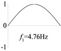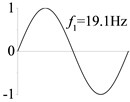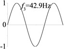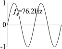
2 ( $k_{t 1} = k_{t 2} =$ 1.2×10⁸, $k_{r 1} = k_{r 2} = 0$ , transverse mode)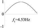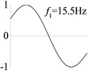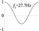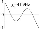
3 ( $k_{t 1} = k_{t 2} = 0.6×1 0^{8}$ , $k_{r 1} = k_{r 2} = 0$ , transverse mode)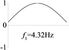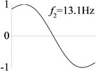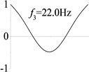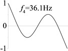
4 ( $k_{t 1} = k_{t 2} = \infty$ , $k_{r 1} = k_{r 2} = 1.7×1 0^{8}$ , transverse mode)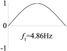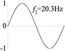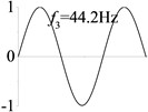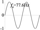
5 ( $k_{t 1} = k_{t 2} = \infty$ , $k_{r 1} = k_{r 2} = 3.4×1 0^{8}$ , transverse mode)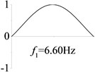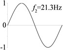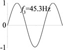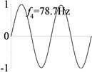
6 ( $k_{a 1} = \infty$ , $k_{a 2} = 0$ , longitudinal mode)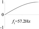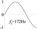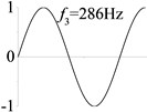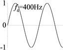
7 ( $k_{a 1} = 1.5×1 0^{7}$ , $k_{a 2} = 0$ , longitudinal mode)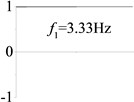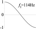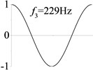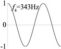
8 ( $k_{a 1} = 1.5×1 0^{6}$ , $k_{a 2} = 0$ , longitudinal mode)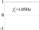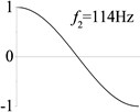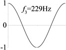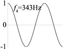

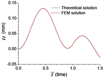
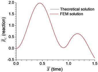
When a moving axial load is applied on the beam with axial spring, as shown in Example 8, the axial displacement and reaction on the boundary node (C and D in Fig. 1) deserve attention [16, 21], which are calculated and shown in Fig. 4. The dimensionless reaction, ${\bar{R}}_{C}$ in Fig. 4(b) is defined as:

62

{\bar{R}}_{C} = \frac{R_{C}}{{R_{C}}_{0}},

where $R_{C}$ is the dynamic reaction on the node C, and ${R_{C}}_{0}$ is the static one, that is 100 Newton in Example 8.

Fig. 2Comparison of mid-span response of the beam with transverse boundary spring under moving load of v=0.1vcr in Example 3: a) dimensionless deflection, b) dimensionless bending moment

Comparison of mid-span response of the beam with transverse boundary spring under moving load of v=0.1vcr in Example 3: a) dimensionless deflection, b) dimensionless bending moment

a)

b)

Fig. 3Comparison of mid-span response of the beam with rotational boundary spring under moving load of v=0.1vcr in Example 4: a) dimensionless deflection, b) dimensionless bending moment

Comparison of mid-span response of the beam with rotational boundary spring under moving load of v=0.1vcr in Example 4: a) dimensionless deflection, b) dimensionless bending moment

a)

b)

Fig. 4Comparison of axial response on the boundary node C of the beam with axial spring under moving load of v=0.1vcr in Example 8: a) axial displacement, b) dimensionless axial reaction

Comparison of axial response on the boundary node C of the beam with axial spring under moving load of v=0.1vcr in Example 8: a) axial displacement, b) dimensionless axial reaction

a)

b)

Fig. 2-4 show that the results from analytical solutions are close to that from FEM analyses, that indicates the methods and equations proposed in this paper is reliable. But in most cases, this analytical solution is used to prove the reliability of FEM analysis. The accuracy of FEM analysis depends on the mesh density, the numerical integration method and the number of mode adopted, while the accuracy of current analytical solution is only related to the number of mode adopted. When the number of mode is sufficient, the current analytical solution for dynamic response of the beam can be considered as an exact solution.

3.2. Effects of the boundary springs

To explore the effects of the elastic boundary constraints on the dynamic response of the beam, forced vibration of the beam with different boundary springs in Table 2 are performed by using the presented analytical method, and the transverse and longitudinal vibration are calculated, respectively.

3.2.1. Effect of the transverse boundary spring on the transverse vibration

Examples 1-3 are calculated to explore the effect of the transverse boundary spring. The modes and natural frequencies in Table 3 indicate that the transverse boundary spring decreases the natural frequency of the beam, and smaller spring coefficient leads to lower natural frequency. The vibration modes of the beams with transverse boundary spring (Examples 2 and 3) are different with that of the simple-supported beam (Example 1) because of the vertical elastic bearing at the boundary.

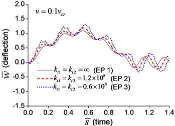
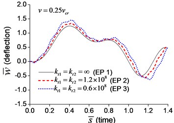
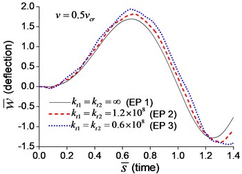
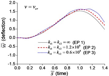
When a moving transverse load is applied on the beam in Examples 1-3, the dimensionless mid-span deflections are calculated and shown in Fig. 5, in which four typical velocities, $0.1 v_{c r}$ , $0.25 v_{c r}$ , $0.5 v_{c r}$ and $v_{c r}$ , are adopted. Fig. 5 indicates that the deflection of the beam with transverse boundary springs (Examples 2 and 3) is larger than that of the simple-supported beam (Example 1), and lower spring coefficient leads to larger deflection of the beam. When the dimensionless time, $\bar{s}$ , is between 0 and 1, the moving load is applying on the beam. Fig. 5 also shows that the higher the velocity of the moving load, the shorter the time of the load passing through the beam, and the more times the beam vibrates while the moving load is applying on.

Fig. 5Mid-span deflection of the beam with transverse boundary springs under moving load of different velocities: a) v=0.1vcr, b) v=0.25vcr, c) v=0.5vcr, d) v=vcr

Mid-span deflection of the beam with transverse boundary springs under moving load of different velocities: a) v=0.1vcr, b) v=0.25vcr, c) v=0.5vcr, d) v=vcr

a)

b)

c)

d)

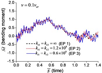
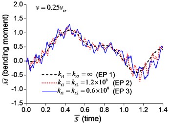
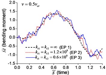
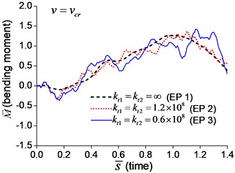
The dimensionless mid-span bending moments are shown in Fig. 6. It indicates that the mid-span bending moment of the beam with transverse springs have more fluctuation than that of the simple-supported beam, which is caused by the vibration of boundary nodes.

Fig. 6Mid-span bending moment of the beam with transverse boundary springs under moving load: a) v=0.1vcr, b) v=0.25vcr, c) v=0.5vcr, d) v=vcr

a)

b)

c)

d)

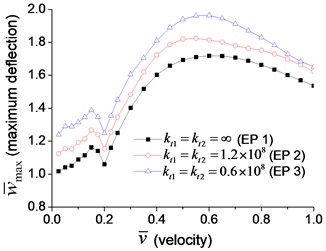
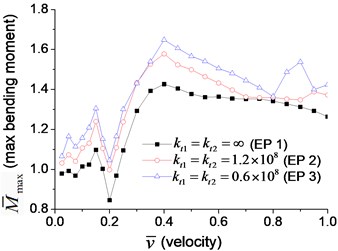
Fig. 7Maximum dimensionless deflection and bending moment of the beam with transverse boundary spring at the velocity varying from 2.5 % to 100 % of critical velocity: a) deflection, b) bending moment

Maximum dimensionless deflection and bending moment of the beam with transverse boundary spring at the velocity varying from 2.5 % to 100 % of critical velocity: a) deflection, b) bending moment

a)

b)

To explore the effect of the velocity of the moving load more clearly, a series of transverse vibration analyses are performed for the velocity ranging from 2.5 % to 100 % of the critical velocity. The maximum dimensionless mid-span deflection and bending moment are shown in Fig. 7(a) and Fig. 7(b), respectively, in which the dimensionless velocity is defined as:

63

\bar{v} = \frac{v}{v_{c r}} .

There are two peaks in Fig. 7(a), and the maximum dimensionless deflection occurs when the velocity is about half the critical velocity. This phenomenon can be explained by the relationship between the time the moving load passes the beam, $L / v$ , and the first-order natural vibration period of the beam, $1 / f_{1}$ . When they are equal to each other, the vibration of the beam struck by the moving load is usually most severe, and the velocity of moving load is $f_{1} L$ , which is half of the critical velocity in Eq. (56). Fig. 7(a) also indicates that lower coefficient of boundary transverse spring (Example 3) means larger maximum bending moment. The trend of the maximum bending moment in Fig. 7(b) is similar to that of maximum deflection in Fig. 7(a), but the curves are rougher, and the maximum bending moment, which is proportional to the second derivative of the deflection, occurs at a lower velocity.

3.2.2. Effect of the rotational boundary spring on the transverse vibration

Examples 1, 4, 5 are calculated to explore the effect of the rotational boundary spring. The modes and natural frequencies in Table 3 indicate that the rotational boundary spring increases the natural frequency of the beam, and larger spring coefficient leads to higher natural frequency. The vibration modes of the beam with rotational boundary springs in Examples 4 and 5 are similar with that of the simple-supported beam in Example 1 except for a slight decrease of rotational angle at the boundary.

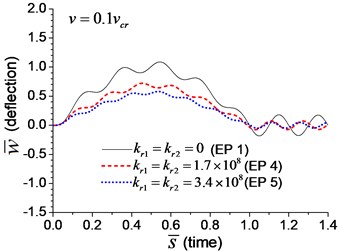
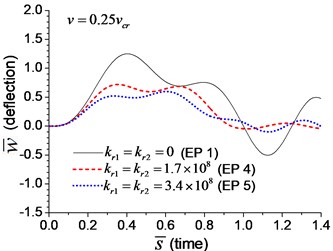
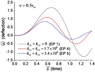
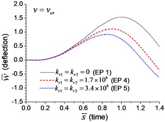
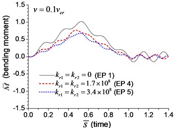
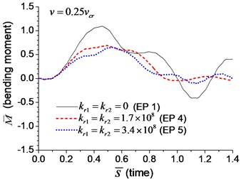
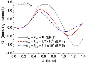
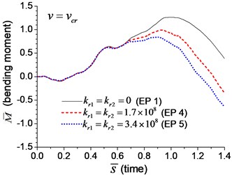
When the moving transverse load is applied on the beam, the dimensionless mid-span deflection is shown in Fig. 8, in which four typical velocities of moving load are adopted. It is obvious that the deflection of the beam with rotational boundary spring (Examples 4 and 5) is smaller than that of the simple-supported spring (Example 1), and higher spring coefficient leads to smaller deflection. The dimensionless mid-span bending moments are shown in Fig. 9. The bending moment of the beam with rotational boundary spring (Examples 4 and 5) is also smaller than that of the simple-supported beam (Example 1), and higher spring coefficient leads to smaller bending moment. It is caused by the negative bending moment at the boundary nodes, C and D in Fig. 1, which decrease the mid-span bending moment.

Fig. 8Mid-span deflection of the beam with rotational boundary springs under moving load of different velocities: a) v=0.1vcr, b) v=0.25vcr, c) v=0.5vcr, d) v=vcr

Mid-span deflection of the beam with rotational boundary springs under moving load of different velocities: a) v=0.1vcr, b) v=0.25vcr, c) v=0.5vcr, d) v=vcr

a)

b)

c)

d)

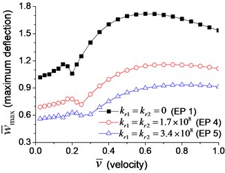
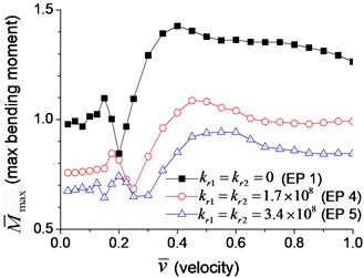
A series of transverse vibration analyses are performed to explore the effect of the velocity of the moving load. The maximum dimensionless mid-span deflection and bending moment are shown in Fig. 10(a) and Fig. 10(b), respectively. Fig. 10 indicates that the maximum mid-span deflection and bending moment fluctuate with the increase of the velocity of moving load, and there are two peaks in the figures. The deflection and bending moment of the beam with boundary rotational spring (Examples 4 and 5) reach the maximum value at higher velocity of moving load than that of simple-supported beam (Example 1), and larger rotational spring coefficient leads to higher velocity in which the maximum deflection and bending moment appear. It is caused by the higher natural frequency of the beam with boundary rotational springs, that increase the critical velocity of moving load.

Fig. 9Mid-span bending moment of the beam with rotational boundary springs under moving load: a) v=0.1vcr, b) v=0.25vcr, c) v=0.5vcr, d) v=vcr

a)

b)

c)

d)

Fig. 10Maximum dimensionless deflection and bending moment of the beam with rotational boundary moment: a) deflection, b) bending moment

a)

b)

3.2.3. Effect of the axial boundary spring on the longitudinal vibration

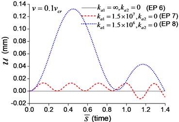
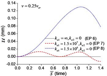
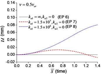
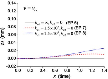
Examples 6-8 are presented to explore the effect of the axial boundary spring. The modes and natural frequencies of longitudinal vibration are shown in Table 3. Since the coefficient of axial boundary springs in Examples 7, 8 are much smaller than the axial stiffness of the beam, the first natural frequency that only depends on the axial boundary spring is much smaller than the other frequencies that depend on the axial stiffness of the beam. If the coefficient of axial boundary spring is close to the axial stiffness of the beam, such as the fixed axial constraint in Example 6, the modes and natural frequencies of the beam depends on both the axial boundary spring and the axial stiffness of the beam.

When the moving axial load is applied on the beam, the axial displacement and reaction on the boundary node C (Fig. 1) are calculated and shown in Figs. 11, 12, in which four typical velocities of moving load are adopted. The critical velocity ( $v_{c r}$ ) of 184 m/s in the transverse vibration is used in this section. It should be noted that this velocity is only used for scaling the velocity, not the critical velocity for the moving axial load.

Fig. 11Axial displacement on the boundary node C of the beam under moving load of different velocity: a) v=0.1vcr, b)v=0.25vcr, c) v=0.5vcr, d) v=vcr

a)

b)

c)

d)

As shown in Figs. 11, 12, the axial displacement and reaction of the beam with axial boundary spring are higher than those of the beam fixed axially in one end. Fig. 11 also shows that smaller coefficient of axial spring leads to larger axial displacement. Fig. 12 indicates that the maximum axial reaction of the beam with axial boundary spring is twice of the static reaction, and much higher than that of the beam fixed axially in one end.

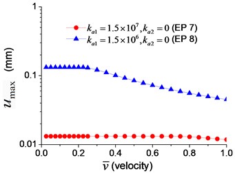
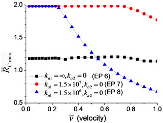
To explore the effect of the velocity of the moving axial load, a series of longitudinal vibration of the beam is analyzed. The maximum displacement and dimensionless reaction on the boundary node C (Fig. 1) are shown in Fig. 13. Fig. 13(a) indicates that smaller spring coefficient (Example 8) leads to larger axial displacement. Fig. 13(b) indicates that the maximum reaction of the beam with axial boundary spring is 2, that is much higher than that of the beam fixed axially in one end, about 1.2.

3.3. Vibration of the beam under an arbitrary moving load

To show the validity of the vibration analysis of the beam under arbitrary moving load in section 2, Examples 9 and 10 in Table 3 are analyzed. The function of the moving transverse and axial loads in these two examples are both:

64

P = \{\begin{array}{l} 100 t, 0 \leq t < T / 2, \\ 50 T, T / 2 \leq t \leq T . \end{array}

Fourier series of this function is:

65

P (t) = 37.5 T + \sum_{n = 1}^{N} \{\frac{50 T}{n^{2} π^{2}} [{(- 1)}^{n} - 1] c o s \frac{2 n π (t - T)}{T} - \frac{50 T}{n π} s i n \frac{2 n π (t - T)}{T}\} .

The transverse and axial vibrations of the beam are calculated respectively as follows.

Fig. 12The axial reaction on the boundary node C of the beam under moving load of different velocity: a) v=0.1vcr, b) v=0.25vcr, c) v=0.5vcr, d) v=vcr

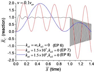
a)

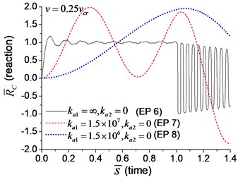
b)

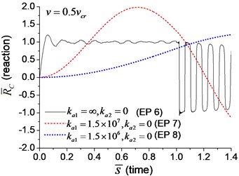
c)

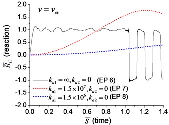
d)

Fig. 13Maximum axial displacement and dimensionless reaction at the velocity varying from 5 % to 100 % of vcr: a) axial displacement, b) axial reaction

a)

b)

3.3.1. Transverse vibration

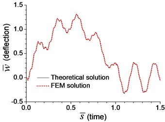
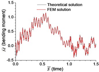
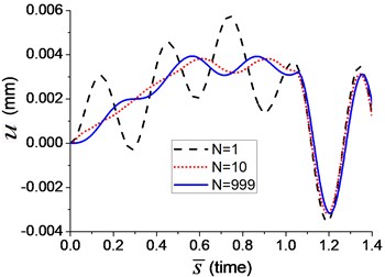
Two velocities of moving load, 18.4 m/s and 184 m/s, i.e. $0.1 v_{c r}$ and $v_{c r}$ , are adopted in the transverse vibration analysis for Example 9. The mid-span deflection of the beam is shown in Fig. 14, in which three curves reflect the deflections when the number of the terms in Fourier series, N, is 1, 10 and 999, respectively. It indicates that more terms in Fourier series means higher accuracy of the simulation. The curve of deflection has converged to a stable one when $N$ equals 999.

Fig. 14The transverse vibration of the beam under arbitrary moving transverse load represented by Fourier series: a) v=0.1vcr, b) v=vcr

a) $v = 0.1 v_{c r}$

b) $v = v_{c r}$

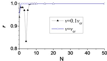
To show the effect of the number of terms clearly, Pearson’s correlation coefficient [22], $r$ is used to measure the accuracy of deflection with different number of terms in Fourier series, while the deflection when $N$ equals 999 is looked as a standard one. The relationship between the Pearson's correlation coefficient and the number of terms in Fourier series, $N$ is shown in Fig. 15. Accurate results are obtained when the Pearson’s correlation coefficient equals 1. Fig. 15 shows that the accuracy of the calculated deflection increases along with the number of terms in Fourier series. The Pearson’s correlation coefficient with the velocity of $v_{c r}$ converges to 1 more rapid than that with the velocity of $0.1 v_{c r}$ . It indicates the deflection with higher velocity of moving load requires less number of terms in Fourier series. This is caused by the shorter time of the moving load spent in passing through the beam at higher velocity, which increases the convergence of Fourier series in Eq. (13).

Fig. 15Pearson’s correlation coefficient (r) of deflection with different number of terms (N) in Fourier series of moving load

3.3.2. Axial vibration

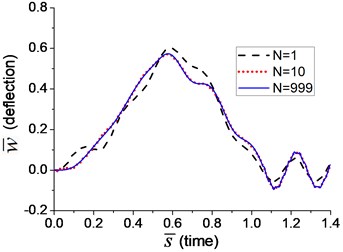
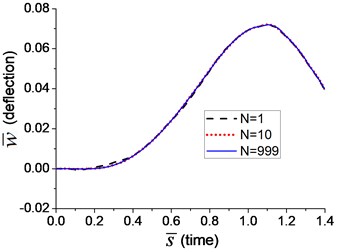
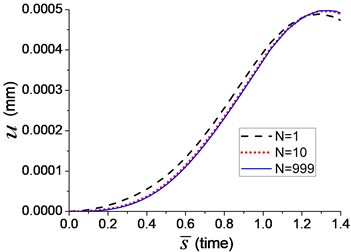
Two velocities of moving load, $0.1 v_{c r}$ and $v_{c r}$ , are also adopted in the axial vibration analysis in Example 13. The axial displacement of the node C (Fig. 1) is shown in Fig. 16, in which three curves represent the displacement when the numbers of the terms of Fourier series, $N$ equals to 1, 10 and 999, respectively. It indicates that more terms in Fourier series leads to higher accuracy of simulation. The curve of displacement has converged to a stable one when $N$ equals 999.

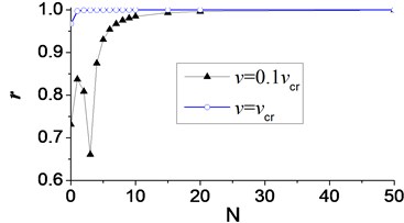
Pearson’s correlation coefficient is also used to measure the accuracy of axial displacement of node C with different number of terms in Fourier series, and the displacement when $N$ equals 999 is looked as a standard one. The relationship between the Pearson’s correlation coefficient and the number of terms in Fourier series is shown in Fig. 17. The accuracy of the calculated displacement also increases along with the number of terms in Fourier series, and the displacement with higher velocity of moving load requires less number of terms.

Fig. 16The axial vibration of the beam under arbitrary moving load represented by Fourier series: a) v=0.1vcr, b) v=vcr

a) $v = 0.1 v_{c r}$

b) $v = v_{c r}$

Fig. 17Pearson’s correlation coefficient (r) of displacement of node C in axial vibration

4. Conclusions

This paper presents an exact solution for the vibration of the beam with multi-directional elastic boundary constraints due to an arbitrary moving load in engineering. After numerical simulation in examples, the following conclusions can be drawn.

1) A closed-form explicit solution is provided for the transverse and axial vibrations of the beam with transverse, rotational and axial boundary springs subjected to a moving load, and this analytical solution can be applied in multiple engineering fields to obtain accurate structural vibrations or to validate the numerical analysis.

2) Smaller coefficient of the transverse boundary spring or rotational boundary spring leads to lower natural frequencies, larger mid-span deflection and bending moment of the beam in the transverse vibration due to moving load.

3) Smaller coefficient of the axial boundary spring leads to lower natural frequencies, larger axial displacement of the beam in the longitudinal vibration due to moving axial load, but the maximum axial reaction on the boundary node remains twice of the static load.

4) The accuracy of calculated deflection of beam due to an arbitrary moving load increases along with the number of terms in Fourier series, and the deflection with higher velocity of moving load required less number of terms in Fourier series.

References

Ouyang H. J. Moving-load dynamic problems: a tutorial (with a brief overview). Mechanical Systems and Signal Processing, Vol. 25, Issue 6, 2011, p. 2039-2060.

Publisher
Heshmati M., Yas M. H. Dynamic analysis of functionally graded multi-walled carbon nanotube-polystyrene nanocomposite beams subjected to multi-moving loads. Materials and Design, Vol. 49, 2013, p. 894-904.

Publisher
Ding Y., Huang Q., Huang J. Y. Theoretical analysis for the static and dynamic characteristics of multisimple-span bridges with continuous deck. Engineering Mechanics, Vol. 32, Issue 9, 2015, p. 100-110.

Search CrossRef
Timoshenko S. P. On the forced vibration of bridges. Philosophical Magazine, Vol. 43, Issue 6, 1922, p. 1018-1019.

Publisher
Fryba L. Vibration of Solids and Structures under Moving Loads. Third Edition, Thomas Telford, London, 1999.

Publisher
Hilal M. A., Zibden H. S. Vibration analysis of beams with general boundary conditions traversed by a moving force. Journal of Sound and Vibration, Vol. 229, Issue 2, 2000, p. 377-388.

Publisher
Hilal M. A., Mohsen M. Vibration of beams with general boundary conditions due to a moving harmonic load. Journal of Sound and Vibration, Vol. 232, Issue 4, 2000, p. 703-717.

Publisher
Yang J., Chen Y., Xiang Y., et al. Free and forced vibration of cracked inhomogeneous beams under an axial force and a moving load. Journal of Sound and Vibration, Vol. 312, Issues 1-2, 2008, p. 166-181.

Publisher
Ouyang H. J., Wang M. J. A dynamic model for a rotating beam subjected to axially moving forces. Journal of Sound and Vibration, Vol. 308, Issues 3-5, 2007, p. 674-682.

Publisher
Şimşek M., Cansız S. Dynamics of elastically connected double-functionally graded beam systems with different boundary conditions under action of a moving harmonic load. Composite Structures, Vol. 94, Issue 9, 2012, p. 2861-2878.

Publisher
Zhu X. Q., Law S. S. Moving load identification on multi-span continuous bridges with elastic bearings. Mechanical Systems and Signal Processing, Vol. 20, 7, p. 1759-1782.

Publisher
Dmitriev A. S. Longitudinal vibrations of a beam with a moving load. Leningrad Institute of Railroad Transportation Engineers, Vol. 12, Issue 2, 1976, p. 100-105.

Publisher
Mamandi A., Kargarnovin M. H., Younesian D. Nonlinear dynamics of an inclined beam subjected to a moving load. Nonlinear Dynamics, Vol. 60, Issue 3, 2009, p. 277-293.

Publisher
Nguyen V. H., Duhamel D. Finite element procedures for nonlinear structures in moving coordinates. Part 1: Infinite bar under moving axial loads. Computers and Structures, Vol. 84, Issue 21, 2006, p. 1368-1380.

Publisher
Wu J. J. Transverse and longitudinal vibrations of a frame structure due to a moving trolley and the hoisted object using moving finite element. International Journal of Mechanical Sciences, Vol. 50, Issue 4, 2008, p. 613-625.

Publisher
Toth J., Ruge P. Spectral assessment of mesh adaptations for the analysis of the dynamical longitudinal behavior of railway bridges. Archive of Applied Mechanics, Vol. 71, Issues 6-7, 2001, p. 453-462.

Publisher
Ding Y., Zhang W., Au F. T. K. Effect of dynamic impact at modular bridge expansion joints on bridge design. Engineering Structures, Vol. 127, 2016, p. 645-662.

Publisher
Chopra A. K. Dynamics of Structures: Theory and Applications to Earthquake Engineering. Second Edition, Prentice Hall, New Jersey, 2004.

Search CrossRef
Zienkiewicz O. C., Taylor R. L. The Finite Element Method. Sixth Edition, McGraw-Hill, London, 2005.

Publisher
Ding Y., Liang Y. H., Zhang W., et al. A computational method for the traffic vibration and sound radiation of hinged-jointed slab bridge and the analysis of influencing factors. Engineering Mechanics, Vol. 35, Issue 4, 2018, p. 151-159.

Search CrossRef
Chen W. F., Duan L. Bridge Engineering: Substructure Design. CRC Press, Florida, 2003.

Publisher
Rahman N. A. A Course in Theoretical Statistics. Charles Griffin and Company, London, 1968.

Search CrossRef

About this article

Received

24 August 2018

Accepted

05 March 2019

Published

15 November 2019

SUBJECTS

Mechanical vibrations and applications

DOI

https://doi.org/10.21595/jve.2019.20172

Keywords

beam vibration

arbitrary moving load

analytical solution

elastic boundary constraint

multi-directional boundary spring

Acknowledgements

This work has been supported by the National Natural Science Foundation of China (51808301), Natural Science Foundation of Zhejiang Provincial (LY19E080009), and Ningbo Transportation Technology Project (201604).

This is an open access article distributed under the Creative Commons Attribution License, which permits unrestricted use, distribution, and reproduction in any medium, provided the original work is properly cited.

Next article in issue Next

Research article

2020 09 21

Vibration characteristics of Timoshenko stepped beam under moving load considering inertial effect

Shoule Wang, Dan Sun, Hongliang Li

Research article

2018 09 30

Analytical solution for modal analysis of Euler-Bernoulli and Timoshenko beam with an arbitrary varying cross-section

Fatemeh Sohani, H. R. Eipakchi

Research article

2016 12 08

A weak solution for free vibration of multi-span beams with general elastic boundary and coupling conditions

Dongyan Shi, Yue Tian, Kwang Nam Choe, Qingshan Wang

Research article

2015 12 30

Forced transverse vibration analysis of a Rayleigh double-beam system with a Pasternak middle layer subjected to compressive axial load

Nader Mohammadi, Mehrdad Nasirshoaibi

Y. Ding, L. Han, and J. You, “An explicit closed-form solution for transverse and longitudinal vibration of beam with multi-directional elastic constraints under an arbitrary moving load,” Journal of Vibroengineering, Vol. 21, No. 7, pp. 1772–1794, Nov. 2019, https://doi.org/10.21595/jve.2019.20172

Copy Extrica

Copied to clipboard!

TY  - JOUR
DO  - 10.21595/jve.2019.20172
UR  - https://doi.org/10.21595/jve.2019.20172
TI  - An explicit closed-form solution for transverse and longitudinal vibration of beam with multi-directional elastic constraints under an arbitrary moving load
T2  - Journal of Vibroengineering
AU  - Ding, Yong
AU  - Han, Lingxia
AU  - You, Jiuang
PY  - 2019
DA  - 2019/11/15
PB  - JVE International Ltd.
SP  - 1772-1794
IS  - 7
VL  - 21
SN  - 1392-8716
SN  - 2538-8460
ER  - 

Copy Ris

Copied to clipboard!

@article{Ding_2019,
	doi = {10.21595/jve.2019.20172},
	url = {https://doi.org/10.21595/jve.2019.20172},
	year = 2019,
	month = {nov},
	publisher = {{JVE} International Ltd.},
	volume = {21},
	number = {7},
	pages = {1772--1794},
	author = {Yong Ding and Lingxia Han and Jiuang You},
	title = {An explicit closed-form solution for transverse and longitudinal vibration of beam with multi-directional elastic constraints under an arbitrary moving load},
	journal = {Journal of Vibroengineering}
}

Copy Bibtex

Copied to clipboard!

[1]Y. Ding, L. Han, and J. You, “An explicit closed-form solution for transverse and longitudinal vibration of beam with multi-directional elastic constraints under an arbitrary moving load,” Journal of Vibroengineering, vol. 21, no. 7, pp. 1772–1794, Nov. 2019, doi: 10.21595/jve.2019.20172.

Copy IEEE

Copied to clipboard!

Ding, Yong, Lingxia Han, and Jiuang You. “An Explicit Closed-Form Solution for Transverse and Longitudinal Vibration of Beam with Multi-Directional Elastic Constraints under an Arbitrary Moving Load.” Journal of Vibroengineering 21, no. 7 (November 15, 2019): 1772–94. https://doi.org/10.21595/jve.2019.20172.

Copy Chicago

Copied to clipboard!

An explicit closed-form solution for transverse and longitudinal vibration of beam with multi-directional elastic constraints under an arbitrary moving load

Abstract

Highlights

1. Introduction

2. Theory and formulations

2.1. Transverse vibration

2.1.1. Modal analysis of transverse vibration

2.1.2. Forced vibration analysis of transverse vibration

2.2. Longitudinal vibration

2.2.1. Modal analysis of longitudinal vibration

2.2.2. Forced vibration analysis of longitudinal vibration

3. Numerical results and discussion

3.1. Comparison between analytical solutions and FEM analyses

3.2. Effects of the boundary springs

3.2.1. Effect of the transverse boundary spring on the transverse vibration

3.2.2. Effect of the rotational boundary spring on the transverse vibration

3.2.3. Effect of the axial boundary spring on the longitudinal vibration

3.3. Vibration of the beam under an arbitrary moving load

3.3.1. Transverse vibration

3.3.2. Axial vibration

4. Conclusions

References

About this article

Related Articles