Vibration characteristics of Timoshenko stepped beam under moving load considering inertial effect

1. Introduction

In the process of artillery launching, the gravity and eccentricity which is caused by high speed projectile will induce barrel vibration. The coupling vibration between projectile and barrel is an important factor which affects the firing accuracy of artillery [1]. With the development of new artillery, it is necessary to study the barrel vibration caused by the motion of projectile.

Zhou Ding [2] and others obtained a general solution for the lateral vibration of the barrel during single and continuous firing, and established a complete theory and analysis method for the vibration of the barrel caused by the movement in the projectile bore. Peng Xian [3] established the dynamic equations of the artillery system under the motion of the base, and solved them separately using the perturbation method and the numerical method, and proposed an analytical expression for calculating the deflection of the barrel end. Wei Shechun [4] and others fully considered the influence of the barrel on the movement and force of the projectile during the movement of the projectile, used VC ++ to carry out the parametric secondary development of ANSYS / LS-DYNA, and established a projectile launch finite element integration platform to Precision and efficiency of projectile launch dynamic analysis.

Kang Xinzhong [5] treated the barrel as a conical cantilever beam, and derived the finite element equation of motion of the beam element based on the Dalambert principle and the deformed body virtual work principle, and gave the overall mass matrix, damping matrix, stiffness matrix and the set rule of nodal force array. Liu Ning [6] simplified the barrel into a cantilever beam of equal cross-section. The vibration equation of the barrel was established according to the Bernoulli-Euler elementary beam theory, and the vibration equation of the barrel was solved by modal analysis. The built model basically describes the dynamic characteristics of the system, and provides a simple and effective method for studying the coupling problem of projectiles. Su Zhongting [7] applied the finite element method and cantilever beam theory based on the idea of moving load, simplified the barrel into a flexible variable-section cantilever beam, and applied the cylindrical coordinate system to discretize the barrel structure into standard fan-shaped elements. Time-varying dynamic equations of the radial vibration of the barrel under the action of moving projectiles. Ma Jisheng [8] treated the barrel as a cantilever beam on a kinematic support and the projectile as a rigid body. Based on the Kane equation Huston method, a relatively complete dynamic model for studying the coupling problem between projectile and barrel was established. Using this model, the projectile launch process can be analyzed more accurately.

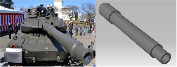
As shown in Fig. 1, the gun barrel can be simplified to a stepped beam. Many researchers have worked on vibration of stepped beams. Mao [9] studied the free vibration of a stepped Euler-Bernoulli beam composed of two uniform sections using the Adomian decomposition method (ADM). Each section is considered a substructure which can be modeled using ADM. Based on the variation method, Su [10] presented an effective formulation for vibration analysis of multiple-stepped functionally graded beams with general boundary conditions. Giunta [11] and Cicirello presented an approach to analyze jointed Euler beams with step changes in material and cross-section under static and dynamic loads. El-Sayed [12] and Farghaly used the normalized transfer matrix (NTM) to derive the exact solution of stepped Timoshenko beam. Yokoyamat [13] considers the effect of axial force, transverse shear deformation and rotational inertia on the Timoshenko beam of equal cross-section. The free vibration equation of Timoshenko beam of equal cross-section is derived from the Hamilton principle, and the natural frequency and mode of the Timoshenko beam are obtained. EI-Sayed [14] solves the natural frequency and mode of a single-span Timoshenko beam of equal cross-section under axial force and proposes a mathematical model for structural engineering. Hu [15] and Wang formed the Hamilton system for solving the dynamic characteristics of the cantilever Timoshenko beam on the basis of considering the effects of shear deformation and rotational inertia.

Fig. 1Simplified diagram of gun barrel

The dynamic problem of beams under moving loads is also a research hot spot. Yang and Wang [16] studied the dynamic response and stability of an inclined beam under a moving vertical concentrated load. They presented the governing equation for transverse motion of the beam. It contained the effect of the compressive axial component of the vertical load on the bending stiffness capacity of the beam. Sudheesh [17, 18] analysed the forced-free responses of nonuniform beams under moving point loads. They presented simple approximate analytical formula for the forced responses of undamped nonuniform beams, which was derived using the fundamental mode by the Rayleigh-Ritz (R-R) method. Saif and David [19] presented a rigorous study on the behaviour of buried pipes under static and moving traffic loads using a robust finite element analysis. Olga [20] analysed the dynamic behaviour of a Rayleigh multi-span uniform continuous beam system that is traversed by a constant moving force. You and Yan [21] concerned with the mechanical responses of anisotropic multi-layered medium under harmonic moving load. Fang [22] established a new track-multilayer ground model to investigate railway subgrade dynamic responses induced by moving train load.

Most articles on gun barrel vibration is based on Euler beam theory. This method has a small scope of application which is only suitable for slender structures [23]. Based on Timoshenko beam theory, the transfer matrix of Timoshenko beam is derived in this paper. The equation of inertia moving load is obtained by analysing the motion of the moving load. The forced vibration of cantilever beam is solved by Newmark method. The influence of mass, speed and acceleration on inertia coefficient is analysed in detail. The modelling and analysis methods adopted in this paper are also applicable to other engineering vibration problems caused by moving loads.

2. The vibration equation of stepped cantilever beam

The primary suppose based on the Euler beam theory is simple. The calculated results are close to the true values when the beam is slender or the low-order frequency is analysed. The Timoshenko beam theory considers the shear deformation and the moment of inertia caused by the bending deformation. It guarantees the accuracy of dynamic parameters of beams when analyse high-order mode or deep beam model. Fig. 2 shows the force and deformation state of the beam micro-unit.

Fig. 2Timoshenko beam micro-unit force and deformation diagram

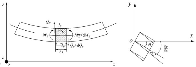
In the Fig. 2, $Q_y$ is the shear, $M_z$ is the moment, $I_q$ is the inertial force acting on the beam micro-unit, $I_0$ is the inertia moment acting on the beam micro-unit, $\gamma$ is the shear angle produced by shear deformation on the neutral axis, $\theta$ is the angle produced by bending, $y$ is the transverse deformation of the beam micro-unit. The inertial force $I_q$ and the inertia moment $I_0$ acting on the beam micro-unit are as shown in the following formulas:

where $\mu$ is the linear density, $I$ is the moment of inertia, and $\rho$ is the density. According to the theoretical mechanics, the dynamic equilibrium equations of beam micro-unit are listed:

According to the material mechanics:

Bring Eq. (3a) and Eq. (3b) into Eq. (2a) and Eq. (2b), then obtain the transverse vibration equation of the Timoshenko beam:

where $E$ is the elastic modulus, $G$ is the shear modulus, $A$ is the cross-sectional area, $k$ is the correction coefficient considering the uneven distribution of shear strain on the section.

Separating $y$ and $\theta$ in Eq. (4a) and Eq. (4b) to obtain a new system of equations:

Supposing the system performs the same-frequency harmonic motion $y(x,t)=y\left(x\right)\mathrm{s}\mathrm{i}\mathrm{n}\omega t$. Where $\omega$ is the free vibration angular frequency of the system, $y\left(x\right)$ is mode shape function. Bring $y\left(x,t\right)$ into Eq. (5a):

where $g$ and $a$ are intermediate variables:

Supposing the general solution of $y\left(x\right)$:

Bringing Eq. (8) into Eq. (6):

Solving the roots of Eq. (9) are $\pm {\stackrel{-}{\lambda }}_1$ and $\pm i{\stackrel{-}{\lambda }}_2$:

Bringing the obtained root into Eq. (8) and get the general solution of $y\left(x\right)$ as the following equation:

where $C_1$ to $C_4$ are undetermined constants. The fourth-order partial differential equation of $\theta \left(x,t\right)$ is the same as $y\left(x,t\right)$. Therefore, the solution of the fourth-order partial differential equation of $\theta \left(x,t\right)$ is as follow:

where $B_1$ to $B_4$ are undetermined constants. Eq. (11) and Eq. (12) are not independent. Bringing Eq. (11) and Eq. (12) into Eq. (4b), the relationship between $B_1$~$B_4$ and $C_1$~$C_4$ can be obtained by using the condition that the coefficients of $\mathrm{s}\mathrm{i}\mathrm{n}{\stackrel{-}{\lambda }}_{2}x$, $\mathrm{c}\mathrm{o}\mathrm{s}{\stackrel{-}{\lambda }}_{2}x$, $\mathrm{s}\mathrm{i}\mathrm{n}\mathrm{h}{\stackrel{-}{\lambda }}_{1}x$ and $\mathrm{c}\mathrm{o}\mathrm{s}\mathrm{h}{\stackrel{-}{\lambda }}_{1}x$ on both sides of the equation are equal:

Assuming intermediate variables $\alpha$ and $\beta$:

Bringing Eq. (11) and Eq. (12) into Eq. (3a) and Eq. (3b), then can get the following equations:

Combining Eq. (11), (12), (15a), (15b) to establish equations:

Listing the boundary conditions at the left end of the beam:

Bringing the boundary into the Eq. (16):

By introducing Eq. (13a) to Eq. (13d) into the above equation. $C_1$ to $C_4$ can be obtained:

By taking the obtained $C_1$~$C_4$ into the Eq. (16), the entire equations for $y\left(x\right)$, $\theta \left(x\right)$, $Q\left(x\right)$, $M\left(x\right)$ can be obtained. Bringing the boundary conditions at the right end of the beam:

By introducing Eq. (20) into Eq. (16), the transverse vibration transfer matrix of the continuous Timoshenko beam can be obtained:

where [$T$] is the transfer matrix:

Assuming intermediate variables $\sigma$, $\tau$, ${\beta }^4$ and $c_0$-$c_5$:

This gives the transfer matrix [$T$] of a single beam. The transfer matrix of stepped beam can be obtained by multiplying multiple transfer matrices:

The transfer matrix of the step beam is represented by [$H$]:

Bringing cantilever beam boundary conditions:

The transfer matrix of cantilever beam is shown:

The coefficient determinant must be zero as the equation having non-zero solution:

Solving the determinant, the natural frequency $\omega$ of the stepped beam can be obtained. The mode shape functions are obtained by bringing the natural frequency into the Eq. (11) and Eq. (12). Then normalize the mode function, the normal modes $\varphi \left(x\right)$ and $\phi \left(x\right)$ can be obtained. Where $\varphi \left(x\right)$ is transverse displacement mode shape function and $\phi \left(x\right)$ is bending angle mode shape function.

Fig. 3Moving load acceleration analysis diagram

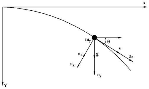
As shown in the Fig. 3, since the beam itself is vibrating, the moving load has a transverse inertial force. When the barrel coupling is not considered, the moving load is only gravity mg. When considering the barrel coupling, the inertia term of the moving load needs to be increased. In the Fig. 3, θ is the bending angle; $v$ is the velocity of the moving load; $a_y$ is the transverse acceleration of the micro-unit due to the bending deformation of the beam; $a_{\tau }$ is the tangential acceleration of the moving load; $a_n$ is the normal acceleration of the moving load; $a_k$ is the Coriolis acceleration caused by the interaction between rotational angular velocity and axial motion velocity.

According to the knowledge of material mechanics and theoretical mechanics:

The actual vertical acceleration of moving load is as follows:

The force acting on the beam by the moving load considering the inertial effect is $P\left(x,t\right)$:

where, $m_y$ represents the mass of the moving load; $s\left(t\right)$ represents the displacement of the moving load. In the Eq. (33), the first term represents the gravitational acceleration. The second term represents the transverse acceleration. The third term represents the Coriolis acceleration. The fourth and fifth terms represent the normal acceleration component and the tangential acceleration component, respectively.

$\delta (x-s(t\left)\right)$ is the Dirac Delta function:

Bring $y(x,t)=\varphi \left(x\right)q\left(t\right)$ and $\theta (x,t)=\varphi \left(x\right)q\left(t\right)$ into the Eq. (33):

In Eq. (35), $i$ represents the $i$th order national frequency. By using the method of separating variables and the orthogonality of modal functions, the integral of the whole beam can be obtained:

By separating and sorting out the terms of zero, primary and secondary derivatives of generalized coordinates in the formula, the [$M$], [$K$], [$C$] matrices of the system are obtained, where [$M$], [$K$], [$C$] are symmetric matrices. The vibration differential equation of the whole system is expressed as follows:

In the above Eq. (37), ${\varphi }_i\left(s\right)$ and ${\phi }_i\left(s\right)$ represent the mode function of the beam where the moving load displacement is $s$. For such time-varying coefficient differential equations, it can only be solved by numerical method of step-by-step integration. Newmark-$\beta$ method is the most commonly used integration method. By calculating the generalized coordinate $q\left(t\right)$ at any time, the dynamic response $y\left(x,t\right)$ of the stepped beam at any time can be obtained.

3. Example analysis and discussion

3.1. Numerical validation

As shown in Fig. 4, a five-stepped beam with a moving load is analysed. In this section, the Timoshenko beam transfer matrix is compared with the Euler beam transfer matrix and FEM calculation results to verify the correctness of the model.

The parameters of the cantilever beam are given in Table 1.

Numerical solutions of Timoshenko beam model and Euler beam model are calculated by programming in MATLAB software. The APDL language of ANSYS software is used in the finite element method for parametric programming. The stepped beam uses the BEAM188 element. The moving load uses the birth-death element. The finite element model is shown in Fig. 5.

The first four natural frequencies are extracted for comparison. The results are shown in the following Table 2.

Fig. 4Five-stepped cantilever beam model diagram

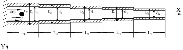
Fig. 5Finite element simulation diagram

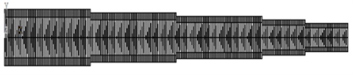
Table 1Model parameter table

$E=$2.1×105 MPa, ${\mu }_P=$ 0.3, $\rho =$7800 kg/m3, $k=$3/4
Section number	Length (m)	Inner diameter (m)	Outer diameter(m)
$L_1$	1.0	0.20	0.4
$L_2$	1.0	0.18	0.35
$L_3$	1.0	0.15	0.30
$L_4$	0.5	0.12	0.25
$L_5$	0.5	0.10	0.20

Table 2Frequency comparison table

	FEM / Hz	Timoshenko beam / Hz	Euler beam / Hz	Timoshenko deviation (%)	Euler deviation (%)
${\omega }_1$	28.45	28.54	28.78	0.32	1.16
${\omega }_2$	118.03	119.13	123.68	0.93	4.79
${\omega }_3$	272.17	276.88	299.63	1.73	10.09
${\omega }_4$	467.72	479.57	544.75	2.53	16.47

It is shown in Table 2 that the difference of the first natural frequency is small. For the following three natural frequencies, the difference between Euler beam and FEM is big. As mentioned in the introduction, the poor calculation accuracy of Euler beams is because each simplified stepped beam belongs to a deep beam structure, and does not consider the section shear deformation and moment of inertia. Therefore, Timoshenko beam has higher accuracy than Euler beam.

The mass of moving load is 10 kg, the speed is 100 m/s. It runs in the beam at a constant speed. The forced vibration of beam is analyzed by Newmark-$\beta$ method. The step length is set to 2×10^-4 s. The Newmark coefficient ${\gamma }_N$ is 0.5, ${\beta }_N$ is 0.25. The response of the free endpoint is extracted as the research object. The calculation results are shown in the following figures.

Fig. 6 shows the time domain response of the free endpoint on the beam. With the movement of the moving load, the displacement of the free endpoint increases. The FEM ’s response is the biggest. The Euler beam’s response is the smallest. Fig. 7 shows the percentage of the difference between the Timoshenko beam model and the Euler beam model for FEM results. Through the error comparison, we can know that Timoshenko beam is more accurate than Euler beam.

The 4 m and 8 m length beams are selected for studying the influence of the beam size on natural frequencies. The dimensions are shown in Table 3.

Fig. 6Response contrast diagram

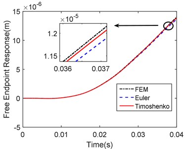
Fig. 7Error percentage contrast diagram

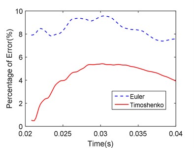
Table 3Beam size parameter table

Beam length	Segment length (m)	Size	Inner and outer diameter parameters (m)
4 m	$L_1=$1, $L_2=$ 1, $L_3=$1, $L_4=$ 0.5, $L_5=$ 0.5	Thick	$D_1=$0.8, $D_2=$0.7, $D_3=$0.6, $D_4=$0.5, $D_5=$0.4, $d_1=$ 0.4, $d_2=$0.36, $d_3=$ 0.3, $d_4=$ 0.24, $d_5=$0.2
		Middling	$D_1=$0.4, $D_2=$0.35, $D_3=$0.3, $D_4=$0.25, $D_5=$0.2 $d_1=$0.2, $d_2=$0.18, $d_3=$ 0.15, $d_4=$ 0.12, $d_5=$0.1
8 m	$L_1=$ 2, $L_2=$2, $L_3=$2, $L_4=$1, $L_5=$1
		Slender	$D_1=$0.2, $D_2=$0.175, $D_3=$ 0.15, $D_4=$ 0.125, $D_5=$0.1 $d_1=$0.1, $d_2=$0.09, $d_3=$0.075, $d_4=$0.06, $d_5=$0.05

The first four natural frequencies are analyzed. The result is shown in Table 4. It can be seen that if the length of the beam is fixed, the smaller the diameter, the smaller the deviation; if the diameter is fixed, the longer the length of the model, the smaller the deviation. The slender the size of the beam, the higher the accuracy of the calculation. The accuracy of the Timoshenko beam model is 3-5 times higher than Euler beam which is greater for higher order natural frequencies. For the slender beam, both theoretical models can solve the problem well. However, if it is a short thick beam or under the high-order natural frequency, the Euler beam model is no longer applicable. For a 4m thick beam, the maximum length-to-diameter ratio of a single segment reached 0.8, the error of the fourth-order frequency of Timoshenko beam is more than 5 %. Therefore, in actual calculation, the diameter of the beam should not be simplified too thick, which makes the calculation accuracy worse.

3.2. Study the effect of moving load single variable on beam vibration

The stepped cantilever beam model in Table 1 is selected for analysis. Moving loads can be divided into considering-inertia-effect and considering-gravity-only. The response of the free endpoint is extracted for analysis. The inertia coefficient ${\lambda }_I$is defined:

38

${\lambda }_I=\left(\left|\frac{y_I-y_g}{y_g}\right|\right)\times 100\mathrm{}\mathrm{\%}.$

In the Eq. (38), $y_I$ represents the response of the free endpoint when the moving load considering inertia effect moving to the free endpoint; $y_g$ is the response of the free endpoint when the moving load only considering gravity moving to the free endpoint.

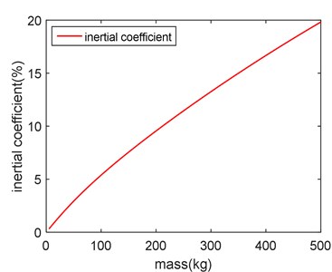
3.2.1. The impact of moving load mass on response results

The influence of mass on the response of the cantilever beam is studied by changing the mass of moving load. The moving load moves uniformly on the beam at the speed of 100 m/s. The mass of the moving load ranges from 5 kg to 500 kg, which the increment is 5 kg. When the moving load moves to the free endpoint, the response of the free endpoint is selected as the research object. The curves obtained are as follows.

Table 4Size effect on frequency table

Beam length	Size	FEM (Hz)	Timoshenko beam (Hz)	Euler beam (Hz)	Timoshenko deviation (%)	Euler deviation (%)
4 m	Thick	55.16	55.62	57.57	0.83	4.37
		210.2	215.94	247.36	2.73	17.68
		444.56	464.18	599.25	4.41	34.80
		709.51	749.94	1089.49	5.70	53.56
	Middling	28.45	28.54	28.78	0.32	1.16
		118.03	119.13	123.68	0.93	4.79
		272.17	276.88	299.63	1.73	10.09
		467.72	479.57	544.75	2.53	16.47
	Slender	14.34	14.36	14.39	0.14	0.35
		61.07	61.24	61.84	0.28	1.26
		145.9	146.65	149.81	0.51	2.68
		260.73	262.77	272.37	0.78	4.46
8 m	Thick	14.23	14.26	14.39	0.21	1.12
		59.02	59.54	61.84	0.88	4.78
		136.09	138.37	149.81	1.68	10.08
		233.86	239.66	272.37	2.48	16.47
	Middling	7.17	7.18	7.2	0.14	0.42
		30.53	30.61	30.92	0.26	1.28
		72.95	73.33	74.91	0.52	2.69
		130.36	131.39	136.19	0.79	4.47
	Slender	3.59	3.59	3.6	0.00	0.28
		15.4	15.42	15.46	0.13	0.39
		37.19	37.25	37.45	0.16	0.70
		67.31	67.46	68.09	0.22	1.16

It can be seen from Fig. 8, the forced vibration response of the free endpoint increases with the increase of moving load mass. The vibration response of the load with inertia effect is smaller than the response only considering gravity, which accords with the result of Eq. (35). As can be seen in Fig. 9, the inertia coefficient increases with the increase of mass. It means that if the mass of moving load is large, the effect of inertia must be considered.

Fig. 8Mass-response contrast diagram

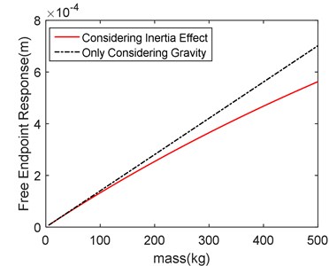
Fig. 9Mass-inertia coefficient diagram

3.2.2. The impact of moving load speed on response results

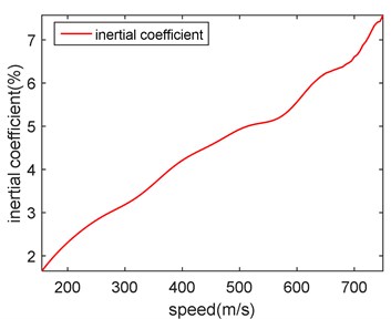
The influence of speed on the response of the cantilever beam is studied by changing the speed of moving load. The moving load moves uniformly on the beam. The mass of the moving load is 10 kg. The speed of the moving load ranges from 150 m/s to 750 m/s, which the increment is 5 m/s. When the moving load moves to the free endpoint, the response of the free endpoint is selected as the research object. The curves obtained are as follows.

It can be seen from Fig. 10, the forced vibration response of the free endpoint decreases gradually with the increase of speed. The vibration response of the load with inertia effect is smaller than the response only considering gravity. It can be known from Eq. (33) that as the speed increases, the amplitude of the excitation force decreases, so the forced response at the free end decreases. As can be seen in Fig. 11, the inertia coefficient increases with the increase of velocity. This means that if the speed of moving load is fast, the effect of inertia must be considered.

Fig. 10Speed-response contrast diagram

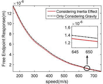
Fig. 11Speed-inertia coefficient diagram

3.2.3. The impact of moving load acceleration on response results

The influence of acceleration on the response of the cantilever beam is studied by changing the acceleration of moving load. The mass of the moving load is 10 kg. The speed is 100 m/s. The acceleration of the moving load ranges from 0 m/s² to 2000 m/s², which the increment is 10 m/s². When the moving load moves to the free endpoint, the response of the free endpoint is selected as the research object. The curves obtained are as follows.

Fig. 12Acceleration-response contrast diagram

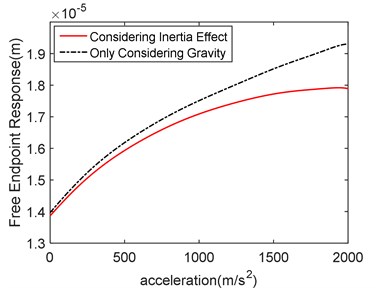
Fig. 13Acceleration-inertia coefficient diagram

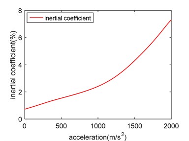
It can be seen from Fig. 12, the forced vibration response of the free endpoint increases with the increase of moving load acceleration. The vibration response of load with inertia effect is smaller than that without inertia effect. As can be seen from Fig. 13, with the increase of the acceleration, the inertia effect coefficient increases accordingly, which means the effect of inertia must be considered if the acceleration of moving load is large. In the range of 0-1000 m/s², the slope of inertia coefficient curve is close to horizontal. At this time, the acceleration has little influence on the inertia effect. When the acceleration exceeds 1000 m/s², the slope of the curve suddenly increases. The acceleration has a great influence on the inertia effect.

3.3. Comparison of double variables of moving load

3.3.1. The impact of the mass and speed of moving load on response results

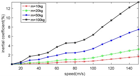
Assume that the moving load performs a uniform motion on the beam. Change the mass and the speed of the moving load. Record the inertia coefficient when the moving load moves to the free endpoint. The results are shown in Fig. 14.

It can be seen from Fig. 14 that both mass and speed affect the value of inertia coefficient. With the mass increases, the value of inertia coefficient increases accordingly. And the same is true of speed to the value of inertia coefficient. The change of mass can significantly change the inertia coefficient. It can be seen from the figure that when the speed is 150 m/s, the inertia coefficient of 100 kg mass is more than twice that of 50 kg mass.

Also, in Fig. 14, when the mass of moving load is large, the influence of inertial effect on vibration response cannot be neglected regardless of the speed. When the mass of moving load is small, the effect of inertia on vibration response at low speed is negligible. However, when the moving load whose mass is 50 kg and speed is 120 m/s, the inertia coefficient exceed 5 %. The inertia effect to the vibration response influence can’t be neglected in this situation.

Fig. 14Inertial coefficient of moving load with different mass and speed

3.3.2. The impact of the mass and acceleration of moving load on response results

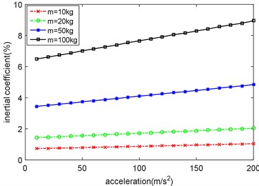
The acceleration analyzed in this paper is uniform acceleration. The influence of inertia effect on vibration response is considered when the moving load performs uniform acceleration motion. Consider the uniform acceleration movement with an initial velocity of 100 m/s. Record the inertia coefficient of the free endpoint. Take the acceleration and mass as variables. Collect multiple sets of data for analysis. The results of uniform acceleration motion are shown in Fig. 15.

As can be seen from Fig. 15, when the mass of the moving load is small, the curve is close to horizontal. At this time, the effect of acceleration on inertia coefficient is negligible. When the mass of the moving load is 10 kg and 20 kg, the inertia coefficient does not exceed 2 %. However, when the mass of the moving load is large, the slope of the curve increases observably. At this time, the influence of acceleration on inertia coefficient cannot be ignored. The inertia coefficient increases consistently with the increase of the speed and the mass. Acceleration has little effect on inertia coefficient in this example. It is only effective at changing the inertia influence coefficient when the mass is large.

Fig. 15Inertial coefficient of moving load with different mass and acceleration

4. Conclusions

Based on the stepped Timoshenko beam model, the transverse vibration response of the cantilever beam under inertial moving loads is analyzed. The conclusions are followed below.

1) Based on Timoshenko beam theory, the transverse vibration transfer matrix is derived in this paper. The equation of the inertia moving load is obtained by analyzing the motion of the moving load. The accuracy of this method is verified by comparing with the Euler beam model and the FEM model. This method can provide theoretical basis for gun barrel vibration.

2) The mass, velocity and acceleration of the moving load all affect the inertia coefficient. The inertia coefficient increases with the increasing mass, velocity and acceleration. This also means that the inertia effect of the moving load must be considered when these three parameters exceed the setting limits. The mass of the moving load is a major factor affecting the inertia coefficient relative to speed and acceleration.