Helicopter landing gear vibration analysis using Lagrange method

Sivakumar, S.

doi:10.21595/vp.2018.20363

Vibroengineering Procedia

Browse Procedia

Published: 13 December 2018

Check for updates

Helicopter landing gear vibration analysis using Lagrange method

S. Sivakumar¹

¹SRM Institute of Science and Technology, Chennai, India

Cite the article Download PDF

Downloads 1821

CrossRef Citations 1

Abstract

In this paper, landing dynamics for a helicopter fitted with an oleo pneumatic landing gear in the front and tail gears has been analysed with a seven degree of freedom mathematical model. Dynamic equations have been developed using Lagrange principle to investigate the effects of vibrations on the structure during landing phase of the helicopter. The bounce, roll, pitch, yaw acceleration response of helicopter landing obtained by numerical simulation in Matlab/Simulink. The developed model by Lagrange method will be useful to measure the vibration levels on landing and taxing of helicopter with uncertainties. This approach is also helpful to optimize the stiffness and damping properties of landing gear.

1. Introduction

Landing is the most critical operational phase of a helicopter. During landing of helicopter on the uneven surface, a large amplitude of vibrations transmitted to the helicopter fuselage structure causing safety and comfort problems to crew and passengers. Moreover, the helicopter also involves complex dynamics of main rotor, tail rotor, engine transmission system and flying dynamics. Landing gear plays an important role in absorbing the shocks and vibrations due to touch down impact and rolling on the deck or un even surface. So, the performance efficiency of the shock absorber is very much essential to meet the variable damping requirements to cope with varying operating conditions. Peter J. F. O. Reilly [1] presented an analytical model for dynamic analysis of landing and taking off of the aircraft from a moving deck. Fu Shang et al. [2] derived the SH-2Fship board dynamic model to prescribe the safe environment for taking off and landing of a helicopter from the flight deck. In his study, energy method used for deriving equations of motion for ship board dynamic motion and assumptions to develop a dynamic model of helicopter. Bernard [3] studied analytic approach of helicopter ship testing simulation for an EH101 helicopter and CPF ship model. Black well and Feik [4] have described a mathematical model of a helicopter landing on an arbitrarily moving deck. The mathematical model of two main oleo and single tail oleo developed and analyzed for oleo load and oleo deflection for deck landing. Kim and Tilbury [5] presented a six degree of freedom mathematical model for a helicopter to investigate the combined action between fly bar and the main rotor blades make it easier for a pilot to fly. Li pan and Chen Renliang [6] presented a helicopter comprehensive analysis by developing a mathematical model with the feature of flexibility and mathematical simplicity. Tulio Salazar [7] developed a mathematical model for a helicopter with a main rotor hub and tail rotor configuration to simulate flying behavior of the helicopter. An active landing gear behavior was demonstrated by Sivakumar and Haran [8] by developing six degree of freedom mathematical model of full aircraft with tricycle landing gear configuration. The author has investigated non-linear analysis of oleo pneumatic landing gear in [8]. Most of the papers have shown the two degree of freedom mathematical model of single landing gear. This model does not include pitch, roll and yaw degrees-of-freedom. The effects of longitudinal and lateral interconnections cannot be studied in the two degrees-of-freedom system model. In this study, the seven degree of freedom math’s model of helicopter with landing gear has been developed using Lagrange method for landing dynamics of helicopter.

2. Mathematical model formulation

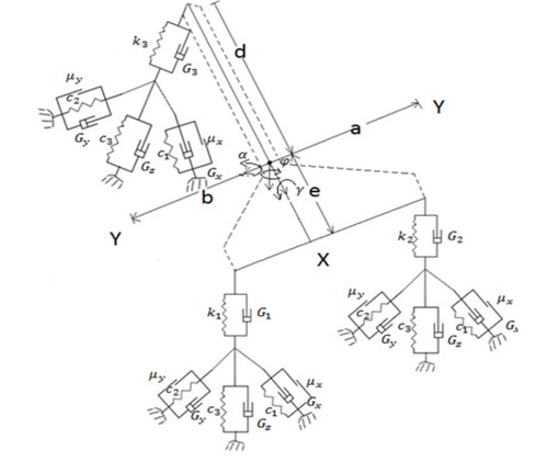
The full helicopter dynamic model built by considering typical US-Navy sea hawk helicopter version. The helicopter fuselage body or concentrated mass $M$ is free to bounce, roll, pitch and yaw. The fuselage mass $M$ is connected to the three lumped masses $m_{t}$ , $m_{l}$ and $m_{r}$ which are tail, front left and front right landing gears piston and tire viewed from front. The front landing gears are called left and right main landing gears and the rear one is called tail landing gear. They are free to bounce vertically with respect to the fuselage mass. The full helicopter model contains four degrees-of-freedom for the helicopter fuselage mass (bounce, roll, pitch, yaw), and three degrees-of freedom for the vertical motions of the tail landing gear tire mass and for the front main landing gears tire masses. In this work, the seven degrees-of-freedom vibration model of the full helicopter as indicated in figure1.This model represents bounce, pitch, roll and yaw motion of the helicopter as $x$ , $α$ , $γ$ , $φ$ about the axes respectively. The displacements and ground excitations of the left, right and tail main landing gears as $x_{1}$ , $x_{2}$ , $x_{3}$ and $y_{1}$ , $y_{2}$ , $y_{3}$ .

The stiffness and damping constants of left shock strut, right and tail gear shock struts indicated as $k_{1}$ , $k_{2}$ , $k_{3}$ and $G_{1}$ , $G_{2}$ , $G_{3} .$ The stiffness and damping constants of left gear tire, right and tail gear tires is denoted as $c_{1}$ , $c_{2}$ , $c_{3}$ . and $G_{x}$ , $G_{y}$ , $G_{z}$ .The tail landing gear is located at a distance of $d$ from centre of gravity (C.G) position. The main landing gears positioned at $e$ -distance from C.G. $b$ -distance from C.G to left main landing gear. $a$ -distance from C.G to right main landing gear. The dynamic equations have been derived by considering $x$ , $φ$ , $α$ , $γ$ for bounce, yaw motion along vertical axis, pitch about lateral axis and roll about longitudinal axis. In this study, helicopter aerodynamic forces and rotor thrust are not taken in to account. In this work, the helicopter landing dynamics equations are written by using Lagrange principle from the model as in Eqs. (1)-(15).

Fig. 1Mathematical model of helicopter with landing gears

Total kinetic energy ( $K$ ) is calculated as:

1

K = \frac{1}{2} m {\dot{x}}^{2} + \frac{1}{2} I_{x x} {\dot{γ}}^{2} + \frac{1}{2} I_{y y} {\dot{α}}^{2} + \frac{1}{2} I_{z z} {\dot{φ}}^{2} + \frac{1}{2} m_{l} {\dot{x}}_{1}^{2} + \frac{1}{2} m_{r} {\dot{x}}_{2}^{2} + \frac{1}{2} m_{t} {\dot{x}}_{3}^{2} .

Total potential energy ( $U$ ) is calculated as:

2

U = \frac{1}{2} k_{1} {(x - x_{1} - b γ - e α + h φ)}^{2} + \frac{1}{2} k_{2} {(x - x_{2} - a γ - e α + h φ)}^{2} + \frac{1}{2} k_{3} {(x - x_{3} + d α + h γ + j φ)}^{2} + \frac{1}{2} c_{3} (x_{1} - y_{1}) + \frac{1}{2} c_{2} {(x_{1} c o s θ - y_{1} c o s θ)}^{2} + \frac{1}{2} c_{1} {(x_{1} c o s θ - y_{1} c o s θ)}^{2} + \frac{1}{2} c_{3} {(x_{2} - y_{2})}^{2} + \frac{1}{2} c_{2} {(x_{2} c o s θ - y_{2} c o s θ)}^{2} + \frac{1}{2} c_{1} {(x_{2} c o s θ - y_{2} c o s θ)}^{2} + \frac{1}{2} c_{3} {(x_{3} - y_{3})}^{2} + \frac{1}{2} c_{2} {(x_{3} c o s θ - y_{3} c o s θ)}^{2} + \frac{1}{2} c_{1} {(x_{3} c o s θ - y_{3} c o s θ)}^{2} + μ_{x} R_{N} (x_{1} c o s θ - y_{1} c o s θ) + μ_{y} R_{N} (x_{1} c o s θ - y_{1} c o s θ) + μ_{x} R_{N} (x_{2} c o s θ - y_{2} c o s θ) + μ_{y} R_{N} (x_{2} c o s θ - y_{2} c o s θ) + μ_{x} R_{N} (x_{3} c o s θ - y_{3} c o s θ) + μ_{y} R_{N} (x_{3} c o s θ - y_{3} c o s θ) .

Total Dissipative energy ( $D$ ) is calculated as:

3

D = \frac{1}{2} G_{1} {(\dot{x} - {\dot{x}}_{1} - b \dot{γ} - e \dot{α} + h \dot{φ})}^{2} + \frac{1}{2} G_{2} {(\dot{x} - {\dot{x}}_{2} - a \dot{γ} - e \dot{α} + h \dot{φ})}^{2} + \frac{1}{2} G_{3} {(\dot{x} - {\dot{x}}_{3} + d \dot{α} + h \dot{γ} + j \dot{φ})}^{2} + \frac{1}{2} G_{z} {({\dot{x}}_{1} - {\dot{y}}_{1})}^{2} + \frac{1}{2} G_{y} {({\dot{x}}_{1} c o s θ - {\dot{y}}_{1} c o s θ)}^{2} + \frac{1}{2} G_{x} {({\dot{x}}_{1} c o s θ - {\dot{y}}_{1} c o s θ)}^{2} + \frac{1}{2} G_{z} {({\dot{x}}_{2} - {\dot{y}}_{2})}^{2} + \frac{1}{2} G_{y} {({\dot{x}}_{2} c o s θ - {\dot{y}}_{2} c o s θ)}^{2} + \frac{1}{2} G_{x} {({\dot{x}}_{2} c o s θ - {\dot{y}}_{2} c o s θ)}^{2} + \frac{1}{2} G_{z} {({\dot{x}}_{3} - {\dot{y}}_{3})}^{2} + \frac{1}{2} G_{y} {({\dot{x}}_{3} c o s θ - {\dot{y}}_{3} c o s θ)}^{2} + \frac{1}{2} G_{x} {({\dot{x}}_{3} c o s θ - {\dot{y}}_{3} c o s θ)}^{2} .

By applying Lagrange method:

4

\frac{d}{d t} (\frac{\partial K}{\partial {\dot{q}}_{k}}) - \frac{\partial K}{\partial q_{k}} + \frac{\partial D}{\partial {\dot{q}}_{k}} + \frac{\partial U}{\partial q_{k}} = Q_{k},

q_{k} = f (x, x_{1}, x_{2}, x_{3}, γ, α, φ, y_{1}, y_{2}, y_{3}),

{\dot{q}}_{k} = f (\dot{x}, {\dot{x}}_{1,} {\dot{x}}_{2}, {\dot{x}}_{3}, \dot{γ}, \dot{α}, \dot{φ}, {\dot{y}}_{1}, {\dot{y}}_{2}, {\dot{y}}_{3}),

5

\frac{d}{d t} (\frac{\partial K}{\partial {\dot{q}}_{k}}) = m \ddot{x} + I_{x x} \ddot{γ} + I_{y y} \ddot{α} + I_{z z} \ddot{φ} + m_{l} {\ddot{x}}_{1} + m_{r} {\ddot{x}}_{2} + m_{t} {\ddot{x}}_{3},

6

\frac{\partial D}{\partial q_{k}} = - G_{1} b \dot{x} + G_{1} b {\dot{x}}_{1} + G_{1} b^{2} \dot{γ} + G_{1} b e \dot{α} - G_{1} b h \dot{φ} - G_{1} \dot{x} e + G_{1} {\dot{x}}_{1} e + G_{1} b e \dot{γ}

- G_{1} h e \dot{φ} + G_{1} e^{2} \dot{α} + G_{1} \dot{x} h - G_{1} {\dot{x}}_{1} h - G_{1} b \dot{γ} h - G_{1} e \dot{α} h + G_{1} h^{2} \dot{φ} + G_{2} a \dot{x} - G_{2} a {\dot{x}}_{2}

+ G_{2} a^{2} \dot{γ} - G_{2} a e \dot{α} + G_{2} a h \dot{φ} - G_{2} \dot{x} e + G_{2} {\dot{x}}_{2} e - G_{2} a e \dot{γ} - G_{2} h e \dot{φ} + G_{2} e^{2} \dot{α} + G_{2} \dot{x} h

- G_{2} {\dot{x}}_{2} h + G_{2} a \dot{γ} h - G_{2} e \dot{α} h + G_{2} h^{2} \dot{φ} - G_{3} d \dot{x} + G_{3} d {\dot{x}}_{3} - G_{3} d h \dot{α} - G_{3} d h \dot{γ} + G_{3} d j \dot{φ}

+ G_{3} d^{2} \dot{α} + G_{3} \dot{x} r - G_{3} {\dot{x}}_{3} r + G_{3} r \dot{γ} h + G_{3} d \dot{α} r + G_{3} r^{2} \dot{φ},

7

\frac{\partial U}{\partial q_{k}} = - k_{1} b x + k_{1} b x_{1} + k_{1} b^{2} γ + k_{1} b e α - k_{1} b h φ - k_{1} x e + k_{1} x_{1} e + k_{1} b e γ - k_{1} h e φ

+ k_{1} e^{2} α k_{1} x h - k_{1} x_{1} h - k_{1} b γ h - k_{1} e α h + k_{1} h^{2} φ + k_{2} a x - k_{2} a x_{2} + k_{2} a^{2} γ - k_{2} a e α

+ k_{2} a h φ - k_{2} x e + k_{2} x_{2} e - k_{2} a e γ - k_{2} h e φ + k_{2} e^{2} α {+ k}_{2} x h - k_{2} x_{2} h + k_{2} a γ h

- k_{2} e α h + k_{2} h^{2} φ + k_{3} h x - k_{3} h x_{3} + k_{3} h^{2} γ + k_{3} d h α + k_{3} r h φ + k_{3} x d - k_{3} x_{3} d

+ k_{3} d h γ + k_{3} d r φ + k_{3} d^{2} α + k_{3} x r - k_{3} x_{3} r + k_{3} r γ h + k_{3} d α r + k_{3} r^{2} φ .

The matrix formulation is written as (8):

8

M \ddot{X} + C \dot{X} + K X = 0,

[M] = [\begin{matrix} M & 0 & 0 & 0 & 0 & 0 & 0 \\ 0 & I_{x x} & 0 & 0 & 0 & 0 & 0 \\ 0 & 0 & I_{y y} & 0 & 0 & 0 & 0 \\ 0 & 0 & 0 & I_{z z} & 0 & 0 & 0 \\ 0 & 0 & 0 & 0 & m_{l} & 0 & 0 \\ 0 & 0 & 0 & 0 & 0 & m_{r} & 0 \\ 0 & 0 & 0 & 0 & 0 & 0 & m_{t} \end{matrix}] \{\begin{matrix} \ddot{x} \\ \ddot{γ} \\ \ddot{α} \\ \ddot{φ} \\ {\ddot{x}}_{1} \\ {\ddot{x}}_{2} \\ {\ddot{x}}_{3} \end{matrix}\} + [C]

= [\begin{matrix} S_{1} & 0 & 0 & 0 & 0 & 0 & 0 \\ 0 & S_{2} & 0 & 0 & 0 & 0 & 0 \\ 0 & 0 & S_{3} & 0 & 0 & 0 & 0 \\ 0 & 0 & 0 & S_{4} & 0 & 0 & 0 \\ 0 & 0 & 0 & 0 & S_{5} & 0 & 0 \\ 0 & 0 & 0 & 0 & 0 & S_{6} & 0 \\ 0 & 0 & 0 & 0 & 0 & 0 & S_{7} \end{matrix}] \{\begin{matrix} \dot{x} \\ \dot{γ} \\ \dot{α} \\ \dot{φ} \\ {\dot{x}}_{1} \\ {\dot{x}}_{2} \\ {\dot{x}}_{3} \end{matrix}\} + [K]

= [\begin{matrix} T_{1} & 0 & 0 & 0 & 0 & 0 & 0 \\ 0 & T_{2} & 0 & 0 & 0 & 0 & 0 \\ 0 & 0 & T_{3} & 0 & 0 & 0 & 0 \\ 0 & 0 & 0 & T_{4} & 0 & 0 & 0 \\ 0 & 0 & 0 & 0 & T_{5} & 0 & 0 \\ 0 & 0 & 0 & 0 & 0 & T_{6} & 0 \\ 0 & 0 & 0 & 0 & 0 & 0 & T_{7} \end{matrix}] \{\begin{matrix} x \\ γ \\ α \\ φ \\ x_{1} \\ x_{2} \\ x_{3} \end{matrix}\} = \{0\},

where:

S_{1} = \dot{x} (- G_{1} b - G_{1} e + G_{1} h + G_{2} a - G_{2} e + G_{2} h - G_{3} d + G_{3} h + G_{3} r),

S_{2} = \dot{γ} (G_{1} b^{2} + G_{1} b e - G_{1} b h + G_{2} a^{2} - G_{2} a e + G_{2} a h - G_{3} d h + G_{3} h^{2} + G_{3} r h),

S_{3} = \dot{α} (G_{1} b e + G_{1} e^{2} - G_{1} e h - G_{2} a e + G_{2} e^{2} - G_{2} e h - G_{3} d + G_{3} d^{2} + G_{3} d h),

S_{4} = \dot{φ} (- G_{1} b h - G_{1} e h + G_{1} h^{2} + G_{2} a h - G_{2} e h + G_{2} h^{2} + G_{3} d r + G_{3} r h + G_{3} r^{2}),

S_{5} = {\dot{x}}_{1} (G_{1} b + G_{1} e - G_{1} h), S_{6} = {\dot{x}}_{2} (- G_{2} a + G_{2} e - G_{2} h), S_{7} = {\dot{x}}_{3} (G_{3} d - G_{3} h - G_{3} r),

T_{1} = x (- k_{1} b - k_{1} e + k_{1} h + k_{2} a - k_{2} e + k_{2} h - k_{3} d + k_{3} h + k_{3} r),

T_{2} = γ (k_{1} b^{2} + k_{1} b e - k_{1} b h - k_{2} a e + k_{2} a h + k_{2} a^{2} + k_{3} h^{2} + k_{3} r h + k_{3} d h),

T_{3} = α (+ k_{1} b e + k_{1} e^{2} - k_{1} e h - k_{2} a e + k_{2} e^{2} - k_{2} e h + k_{3} d^{2} + k_{3} d h + k_{3} d r),

T_{4} = φ (- k_{1} b h - k_{1} h e + k_{1} h^{2} + k_{2} a h - k_{2} e h + k_{2} h^{2} + k_{3} d r + k_{3} r h + k_{3} r^{2}),

T_{5} = x_{1} (k_{1} e - k_{1} h + k_{1} b), T_{6} = x_{2} (- k_{2} a + k_{2} e - k_{2} h), T_{7} = x_{3} (- k_{3} h - k_{3} r - k_{3} d) .

The Eqs. (9)-(15) can be solved separately in Matlab/Simulink as:

9

m \ddot{x} + S_{1} \dot{x} + T_{1} x = 0,

10

I_{x x} \ddot{γ} + S_{2} \dot{γ} + T_{2} γ = 0,

11

I_{y y} \ddot{α} + S_{3} \dot{α} + T_{3} α = 0,

12

I_{z z} \ddot{φ} + S_{4} \dot{φ} + T_{4} φ = 0,

13

m_{l} {\ddot{x}}_{1} + S_{5} {\dot{x}}_{1} + T_{5} x_{1} = 0,

14

m_{r} {\ddot{x}}_{2} + S_{6} {\dot{x}}_{2} + T_{6} x_{2} = 0,

15

m_{t} {\ddot{x}}_{3} + S_{7} {\dot{x}}_{3} + T_{7} x_{3} = 0 .

3. Landing simulation

The Simulink model of typical helicopter with landing gear system has been developed from the dynamic equations written in Section 2 as shown in Fig. 2. Several trials of numerical simulations can be done by using this Simulink model set up. The helicopter of fuselage mass 9000 kg is considered for numerical simulation. The helicopter and landing gear parameters used for numerical simulation has taken from Blackwell and Feik [4] tabulated in Table1 and Table 2.

As per FAR 23.725, recommended free drop height range for both MLG and NLG is minimum 9.2 in and maximum 18.7 in. In this simulation, the higher value of 0.4 m is taken for landing. simulation in Matlab/Simulink environment and landing gear touches the runway at 2.5 s on even ground. During landing simulation both the main landing gears touch first and the tail landing gear later. The vertical acceleration, pitch, roll, yaw acceleration responses due to touch down impact of the main landing gear in time domain is presented in the Fig. 3-6.

Fig. 2Simulation set up in Matlab/Simulink environment

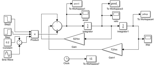
Fig. 3Bounce acceleration response

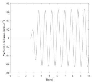
Fig. 4Roll acceleration response

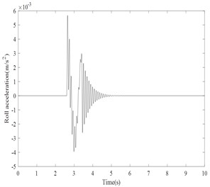
Fig. 5Pitch acceleration response

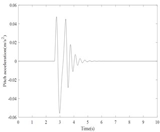
Fig. 6Yaw acceleration response

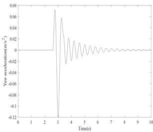
Results shows that vertical acceleration is not settled within a short time. The bounce, roll, pitch and yaw acceleration levels are damped within 2 to 4 secs. The settling time is very less for the helicopter to become stable. The trend of the results for a typical simulation is qualitatively matching with the reference given in [4]. It is very difficult to do the real time experimental validation with the typical helicopter. In future study, the typical helicopter has been developed in other Multi body dynamics software’s like ADAMS or LMS to do landing dynamics.

Table 1Helicopter parameters

Description	Symbol	Value	Units
Helicopter fuselage mass	$M$	9000	kg
Mass moment of inertia about $X X$ axis	$I_{x x}$	9.0e3	kg.m²
Mass moment of inertia about $Y Y$ axis	$I_{y y}$	6.3e4	kg.m²
Mass moment of inertia about $Z Z$ axis	$I_{z z}$	6.0e4	kg.m²
Distance from C.G to tail gear	$d$	3.3	m
Distance from C.G to horizontal axis of main gear	$e$	1.5	m
Distance from C.G to left main landing gear	$a$	1.4	m
Distance from C.G to right main landing gear	$b$	1.4	m

Table 2Helicopter landing gear parameters

Parameter	Main gear	Tail gear	Units	Parameter	Main gear	Tail gear	Units
$k_{1}$	3.6e5	–	N/m	$c_{2}$	4.5e5	6.0e5	N/m
$k_{2}$	5.0e6	–	N/m	$c_{3}$	1.2e6	1.0e6	N/m
$k_{3}$	–	2.0e6	N/m	$G_{x}$	2.0e4	2.0e4	N.s/m
$G_{1}$	2.2e4	–	N.s/m	$G_{y}$	2.0e4	2.0e4	N.s/m
$G_{2}$	4.0e4	–	N.s/m	$G_{z}$	1.0e4	1.0e4	N.s/m
$G_{3}$	–	3.0e4	N.s/m	$μ_{x}$	0.7	0.7	–
$c_{1}$	1.4e6	8.0e5	N/m	$μ_{y}$	0.7	0.7	–

4. Conclusions

In this research work, helicopter with landing gear seven degree of freedom mathematical model using Lagrange method has been developed to investigate dynamic response. The response of bounce, pitch, roll, yaw accelerations are obtained to verify the developed model. The responses are stable. This numerical simulation procedure is helpful to check the vibration levels of aircraft during landing and taxing on the various ground uncertainties. By using this model, the stiffness and damping coefficient of landing gear component obtained experimentally during drop test can be evaluated theoretically. This procedure enables the designer to optimize the design parameters of landing gear in the initial design stage itself for achieving better performance of landing gears.

References

O’Reilly P. J. Aircraft /deck interface dynamics for destroyers. Marine Technology, Vol. 24, Issue 1, 1987, p. 15-25.

Publisher
Me Fu-Shang, Baitis Erich, Myers Milliam Analytical Modeling of SH-2F Helicopter Ship Board Operation. AGARD, AD-A2448690, 1992.

Search CrossRef
Ferrier Bernard, Polvi Henry, Thibodeau Francois A. Helicopter/Ship Analytic Dynamic Interface. AD-A244869, 1992.

Search CrossRef
Black Well J., Feik B. A. A Mathematical Model of the on Deck Helicopter/Ship Dynamic Interface. Aerodynamics Technical Memorandum, AR-005-549, 1988.

Search CrossRef
Kim S. K., Tilbury D. M. Mathematical modeling and experimental identification of a model helicopter. AIAA Modeling and Simulation Technologies Conference and Exhibit, Guidance, Navigation, and Control and Co-located Conferences, 1998.

Publisher
Pan Li, Chen Renliang A mathematical model for helicopter comprehensive analysis. Chinese Journal of Aeronautics, Vol. 23, 2010, p. 320-326.

Publisher
Salazar Tulio Mathematical Model and Simulation for a Helicopter with Tail Rotor, Advances in Computational Intelligence, Man-Machine Systems and Cybernetics. Beijing, China, 2010.

Search CrossRef
Sivakumar S., Haran A. P. Mathematical model and vibration analysis of aircraft with active landing gears. Journal of Vibration and Control, Vol. 21, Issue 2, 2015, p. 229-245.

Publisher
Sivakumar S., Syed Haleem M. Non-linear vibration analysis of oleo pneumatic landing gear at touchdown impact. Mathematical Models in Engineering, Vol. 4, Issue 2, 2018, p. 89-97.

Publisher

Cited by

Blood Product Supply for a Helicopter Emergency Medical Service

(2021)

About this article

Received

11 November 2018

Accepted

22 November 2018

Published

13 December 2018

SUBJECTS

Vibration in transportation engineering

DOI

https://doi.org/10.21595/vp.2018.20363

Keywords

helicopter landing gear

vibration

Lagrange principle

simulation

landing gear properties

This is an open access article distributed under the Creative Commons Attribution License, which permits unrestricted use, distribution, and reproduction in any medium, provided the original work is properly cited.

Previous article in issue Previous Next article in issue Next

Research article

2021 09 09

Investigation of random runway effect on landing of an aircraft with active landing gears using nonlinear mathematical model

S. Sivakumar, T. Selvakumaran, B. Sanjay

Research article

2020 04 02

Promoting both passenger comfort and aircraft handling of 6 DOF landing gear utilizing variable mechanical admittance approach

Mehran Pirooz, Seyed Hossein Mirmahdi, Seyedeh Razieh Moafi

Research article

2018 06 30

Non-linear vibration analysis of oleo pneumatic landing gear at touchdown impact

S. Sivakumar, M. Syedhaleem

Research article

2017 08 15

Numerical simulation and experimental research on aerodynamic noises of the single wheel landing gear in an aircraft

Yao-ming Zhou, Yao-long Liu, Shao-wei Li, Dao-chun Li, Yu-hong Jia

S. Sivakumar, “Helicopter landing gear vibration analysis using Lagrange method,” Vibroengineering PROCEDIA, Vol. 21, pp. 96–101, Dec. 2018, https://doi.org/10.21595/vp.2018.20363

Copy Extrica

Copied to clipboard!

TY  - JOUR
DO  - 10.21595/vp.2018.20363
UR  - https://doi.org/10.21595/vp.2018.20363
TI  - Helicopter landing gear vibration analysis using Lagrange method
T2  - Vibroengineering PROCEDIA
AU  - Sivakumar, S.
PY  - 2018
DA  - 2018/12/13
PB  - JVE International Ltd.
SP  - 96-101
VL  - 21
SN  - 2345-0533
SN  - 2538-8479
ER  - 

Copy Ris

Copied to clipboard!

@article{Sivakumar_2018,
	doi = {10.21595/vp.2018.20363},
	url = {https://doi.org/10.21595/vp.2018.20363},
	year = 2018,
	month = {dec},
	publisher = {{JVE} International Ltd.},
	volume = {21},
	pages = {96--101},
	author = {S. Sivakumar},
	title = {Helicopter landing gear vibration analysis using Lagrange method},
	journal = {Vibroengineering {PROCEDIA}}
}

Copy Bibtex

Copied to clipboard!

[1]S. Sivakumar, “Helicopter landing gear vibration analysis using Lagrange method,” Vibroengineering PROCEDIA, vol. 21, pp. 96–101, Dec. 2018, doi: 10.21595/vp.2018.20363.

Copy IEEE

Copied to clipboard!

Sivakumar, S. “Helicopter Landing Gear Vibration Analysis Using Lagrange Method.” Vibroengineering PROCEDIA 21 (December 13, 2018): 96–101. https://doi.org/10.21595/vp.2018.20363.

Copy Chicago

Copied to clipboard!

Helicopter landing gear vibration analysis using Lagrange method

Abstract

1. Introduction

2. Mathematical model formulation

3. Landing simulation

4. Conclusions

References

Cited by

About this article

Related Articles