Determination of point estimates in an information-measuring system on the basis of light shields

1. Introduction

In different information-measuring systems, including an information-measuring system based on light shields [1, 2] characteristics of random values according to independent samples are important. One of these characteristics is a mathematical expectation. In this case, evaluations for point and interval estimation of for the control of statistical hypotheses are searched [3-5]. Especially in a case of a point and interval estimation the criterion of valuation optimality (statistics $y$($x_1$, …, $x_2$) – the function of sample values $x_1$, …, $x_n$ that does not depend on sample volume $n$) is minimum of its dispersion ${\sigma }^2$. An effective valuation has a minimum amount of dispersion. In the case of a statistical control of hypotheses, the criterion of the optimality is taken the minimum of a total risk (the sums of error probabilities of I kind $\alpha$ and II kind $\beta$), or minimum $\beta$ at a fixed $\alpha$. It is obvious that the smaller a total risk is, the sharper an integral function of evaluation distribution $F\left(y\right)$ is [5, 6].

2. The estimation of a mathematical expectation

Most common random values is distributed to a normal law $N$($\mu$, ${\sigma }^2$) with a mathematical expectation $\mu$ and dispersion ${\sigma }^2$. A wide distribution of a normal law is proved by a central limit theorem of probability theory [4, 5]. Moreover, it follows from the uncertainty principle (entropy according to K. Shennon) in the case of stable test conditions [7]. In the case of a normal random value, its distribution is symmetrical concerning a mathematical expectation, for the valuation of a mathematical expectation we take random average value:

Median ${\overline{x}}_{Me}$ average values $r$ – statistics ${\overline{r}}_{1,n}=\frac{1}{n}\left(x_{\left(1\right)}+x_{\left(n\right)}\right)$, ${\overline{r}}_{2,n-2}=\frac{1}{n}\left(x_{\left(2\right)}+x_{\left(n-1\right)}\right)$ and so on, where $x_{\left(r\right)}$ – $r$-statistics [8].

According to a famous theorem of A. A. Markov [5] an effective (with minimum dispersion) linear estimation (a linear function from random values) of a mathematical expectation at any law of distribution in the case of an independent sampling with equidistant changes is a random average value $\overline{x}$ Eq. (1). The dispersion of valuation $\overline{x}$ is inversely proportional to the sample volume and in the case of small samples ($n$ < 10, …, 20) [9, 10] the problem of the search of more effective valuations in the area of nonlinear functions is actual.

The valuation Eq. (1) follows from the criterion of the optimality according to the least square method (LSM):

A necessary condition of the extremum of the function Eq. (2) at $\theta$, gives a linear valuation Eq. (1). In the case of the criterion of a general view:

If $\nu$ ≠ 2 we get nonlinear valuations, the valuation of least module method (LMM) is a frequent case if $\nu =$ 1 [8].

If $\nu$ > 1, then in the valuation the weights of big deflection are increased, if $\nu$ < 1, then vice versa. So, to take the valuations with $\nu$ > 2 is objectionable. From the point of view of reducing the influence of abnormal measurement, it is appropriate to take the valuations with $\nu$< 1. For defining of valuations on the criterion of a general view the method of variationally weighted quadratic approximation is developed. It can be used only if $\nu$ < 2. If $\nu$ < 1, some problems can appear than can be linked to the presence $n-1$ local (local extremum) function Eq. (3) and dependence of the result of the decision from an initial estimate.

2.1. Determination of the estimation of a mathematical expectation according to the method of least modules

Now we demonstrate, that in the case MLM ($\nu =$ l) the valuation ${\theta }_1$ on the criterion Eq. (3) can be found without using the method of variationally weighted quadratic approximation in a trivial way. ${\theta }_1$ is the valuation of a mathematical expectation in the case of the method Eq. (3) if $\nu =$ 1. We consider the sums of the deflection modules for two extreme $r$-statistics $x_{\left(1\right)}$, $x_{\left(n\right)}$. The dependence of this sum on ${\theta }_1$ has the form, shown in the Fig. 1.

Fig. 1The dependence of the sum of the deflection modules on θ1

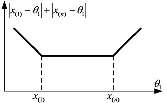
The dependence of the sum of the deflection modules of the following $r$-statistics $x_{\left(2\right)}$, $x_{\left(n-1\right)}$, put in the interval ($x_{\left(1\right)}$, $x_{\left(n\right)}$), has a similar form and the minimum value of a total sum will be within the interval $x_{\left(2\right)}$, $x_{\left(n-1\right)}$ and so on. Thus, the minimum value of the sum will be when ${\theta }_1=x_{\frac{n+1}{2}}$, if $n$ – odd, or in the interval $\left(x_{\left(\frac{n}{2}\right)}+x_{\left(\frac{n+2}{2}\right)}\right)$ if $n$ – even. In this case an optimal value can be taken equal to the middle of the interval ${\theta }_1=\frac{1}{2}\left(x_{\left(\frac{n}{2}\right)}+x_{\left(\frac{n+2}{2}\right)}\right)$. Therefore, MLM-valuation coincides with the median value ${\overline{x}}_{Me}$. From this, it follows that MLM-valuation is an unbiased estimate of a mathematical expectation for symmetric distributions. It concerns other valuations ${\theta }_v$ if $v$ ≠ 2 as well.

Despite the fact that the efficiency of values for $v$ ≠ 2 is smaller, the efficiency of an average value $\theta =\frac{1}{2}\left({\theta }_2+{\theta }_v\right)$ can be close to the efficiency of the value ${\theta }_2=\overline{x}$ thanks to the thing that the correlation coefficient between ${\theta }_2$ and ${\theta }_v$ is not equal to 1. If $v$ ≤ 1, then an average value is less sensitive to abnormal change. In the case if $v=$ 1 the correlation coefficient (when $n$ is odd) between ${\theta }_2=\overline{x}$ by Eq. (1) and $x_{\left(\frac{n+1}{2}\right)}$ is easy to calculate. It is equal to $\rho =-\frac{1}{n-1}$, $n$ ≥ 2 [8].

We also notice that, in the case of hypothesis testing about a mathematical expectation its value for the main hypothesis is known. It removes the problem of the choice of an initial estimate at a finding of an optimal value ${\theta }_v$ Eq. (3). The value:

4

${\theta }_{op}=\frac{1}{2}\left({\theta }_1+{\theta }_2\right)=\frac{1}{2n}{\sum }_r^n{x}_{\left(r\right)}+\frac{1}{2}{x}_{\left(\frac{n+1}{2}\right)}.$

Leads onto the idea to build a linear value of this kind:

5

$\theta ={\sum }_{r=1}^n{c}_r{x}_r,$

where $r$ – statistics are taken with weight coefficients $c_r$.

Coefficients $c_r$ can be calculated, using the MLS-criterion, for example, taking into consideration an additional condition – the immutability of the value. So, the decision brings to the task on a conditional extremum of the function. However, for the decision it is necessary to know the correlation coefficients between $r$ – statistics and their dispersion.

3. Results

On the basis of the analysis of modelling results the following conclusions can be done.

1. Accurate evaluation $z_1$ according to MLM is less effective compared to $y_0$ at the sample mean ($e_{z1}>1$, Table 2). At the same time the approximate evaluation $y_1$ according to MLM, received with the help of the function Minner at an initial estimate, equal to a mathematical expectation is more effective ($e_{y1}<1$, Table 1). If in the case of an initial estimate to take the sample mean $y_0=\overline{x}$, then the effectiveness decreases to about value $e_{z1}$. As a result, approximate evaluations are more effective, and they can be used in the case of checking of statistical hypotheses when a mathematical expectation is supposed known (hypothetically)

2. Accurate evaluations at two or three average members of the sample ($r$ – statistics) according to the effectiveness approach the sample mean (Table 2). Their advantage is insensitivity to abnormal changes.

3. The estimate of standard deviation (e.s.d.) by Eq. (8) is unbiased and by efficiency, it coincides with the value by sample e.s.d.

4. The estimation of a mathematical expectation by Eqs. (9), (10) are unbiased, but by efficiency they concede the value by the sample mean.

5. Values of e.s.d. $\sigma$ by Eqs. (9), (10) are a bit low, the value by Eq. (9) is more accurate. By efficiency the valuations concede the value by the sample mean of e.s.d.

6. An empirical integral function of distribution of average value $y_3$ is sharper than functions of distribution of values $y_0=\overline{x}ny$1. Empirical integral functions of distribution of average point estimates ${zz}_2$, ${zz}_3$ practically coincide with an integral function of distribution of the value $y_0=\overline{x}$.

7. Since the values of coefficients of correlation in the Table 1 are not equal to ±1 (Table 1), then between $y_0$ and $y_1$, as well as between $y_0$ and $y_2$ the dependence is nonlinear.

8. In terms of estimation values of coefficients of correlation in the Table 2, we can conclude that dependences between values $y_0$ and $z_1$, $z_2$, $z_3$ are more linear.

Also, it is necessary to mention that for a normal random value we were not able to find a superefficient nonlinear value [7]. The expediency of using concrete values depends on a situation that is indicated in the work above.

4. Conclusions

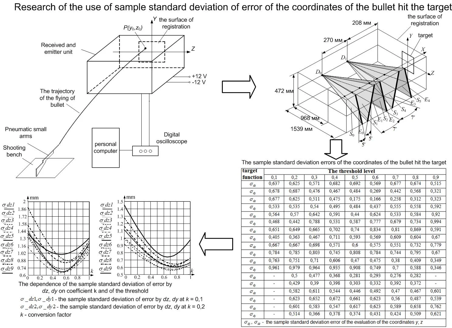
The use of estimates, received in the research process, let raise the accuracy of determination of point estimates when a bullet hits the target in information-measuring systems based on light automatic shields that are intended for small arms testing.

The approximate evaluation of the sample mean $y_1$ is more effective than the accurate evaluation $z_1$ and can be used in the case of statistical hypotheses testing when a mathematical expectation is hypothetically known. If one uses the approximate evaluation of the sample mean, it leads to the rise of the accuracy of determination of point estimates when a bullet hits the target in 1,5 – 2 times. This conclusion is experimentally confirmed in the research [1].

The accurate evaluations of the sample mean by two or more means of the sample are insensible to abnormal measurements and can be used in small arms testing in the conditions of different noises.