Abstract
Bogie is the most important component in a running gear of a high-speed train. Advantages and disadvantages of its mechanical performance can directly influence safety and comfort of train running. Failure of key components on the bogie always leads to serious vibration and performance decrease of each train component, and can even cause serious accidents such as de-railing and overturning. Therefore, it is very necessary to adopt an efficient and accurate intelligent diagnosis method. Based on the previous researches, the paper proposed a deep neural network method to make systematic and complete diagnosis of bogie faults. Firstly, a deep neural network was used to diagnose standard bearing system faults, and the results were compared with those obtained by traditional neural networks such as FANN (Firefly Artificial Neural Network), PSONN (Particle Swarm Optimization Neural Network) and GANN (Genetic Artificial Neural Network) to highlight advantages of the deep neural network. Then, based on vibration data extracted by a multi-body dynamic model of the high-speed train, the deep neural network was used to diagnose 8 conditions of the bogie systematically. The fault diagnosis was repeated for 10 times. Results obtained for the 10 times present obvious advantages of the deep neural network which could obtain the average diagnosis rate of 98.3 % and had the diagnosis standard deviation of 0.71. Finally, training process of fault diagnosis was extracted. Results show that the deep neural network could converge to a critical value at the quickest speed. All the above analysis results indicate that the deep neural network has irreplaceable advantages in intelligent diagnosis of bogies.
1. Introduction
With large-scale acceleration of railway running and operation of high-speed trains, safety and comfort in running of high-speed trains have attracted extensive attention. Sensors distributed at different positions of a high-speed train can detect a lot of data in real time. The data contains a lot of information which can reflect states and train faults. By using the data, generally adaptive features which reflect fault states can be extracted to represent safety states of high-speed trains in the form of feature analysis. It is very important to conduct fault diagnosis.
During high-speed running, key components of a high-speed train may generate faults [1]. Vibration signals monitored by sensors on the high-speed train can reflect whether the running state is normal [2]. Continuous high-speed running of the high-speed train may lead to serious wear and vibration of the running gear. Effective fault diagnosis and recognition of the running gear of high-speed train play an important role in realizing timely maintenance, reducing the use and maintenance cost and guaranteeing train running safety. Current researches on fault features of the train running gear mainly focus on time-frequency analysis of vibration signals, such as wavelet analysis method [3, 4], short-time Fourier transform [5] and empirical mode decomposition [6-8]. All these methods conduct analysis aiming at a single sensor or a single fault. There are many sensors disposed on the running gear of high-speed train, detection data has abundant contents and involves a large scope, and there are many interrelated influential factors on the data, so that the same fault can be described by different feature indexes. Nonlinear mapping is formed between detection amount and fault features, and between the fault features and fault sources. Therefore, diversity and uncertainty of faults and complexity in the correlation between different faults become difficulties in the fault recognition technology [9].
Bogies are the most important component of a running gear of a high-speed train. Mechanical performance of the bogie can directly influence safety and comfort of train running [10]. Failure of key components on the bogie always leads to serious vibration and performance decrease of different train parts, and can even cause serious accidents such as de-railing and overturning. However, current researched aiming at bogie mechanical faults are mainly based on kinetic theories [11, 12]. Due to continuous development of online monitoring systems, a lot of vibration data of train running are obtained [13]. It is very important to carry out data-driven performance monitoring and fault diagnosis of key components of bogies in practical application, where there are a lot of problems needing to be solved.
However, the current fault diagnosis methods require artificial design and selection of bogie fault signal features and are defective in large time consumption, large workloads and low diagnosis accuracy. In recent years, based on the idea of brain learning, Hinton [14, 15] proposed a machine learning method based on deep neural networks. Deep learning is also called as deep neural network [16-18]. The method is a multi-layer non-supervision neural network method, wherein multiple non-linear structures are disposed to complete approaching of a complicated function; the non-supervision learning method can be used to obtain main variables and distribution features of input data. Pang [19] used the deep neural network method to recognize faults of a high-speed train bogie and compared the diagnosis results with those obtained by the BP neural network. However, the research process was not systematic and the feature parameters were incomplete. The research only focused on the condition of single failure of the bogie, and failed to compare diagnosis results of the deep neural network with an improved neural network model. Based on a deep neural network, Xie [20] solved the K-nearest neighbor of an unknown sample on each hidden layer in combination with advantages of KNN (K-Nearest Neighbor), proposed a deep learning algorithm based on K-DBNs and carried out fault diagnosis. However, during the research, the incomprehensive selection of fault features led to low diagnosis accuracy. Guo [21] used a deep belief network to research fault diagnosis under the single failure condition of a bogie. However, the FFT technology was used to transform the time-domain signals of the bogie to the frequency-domain signals. The FFT technology can only be used to process steady signals, where the time-domain signals of bogies are non-steady signals. Yin [22] used the deep neural network method to make real-time monitoring and diagnosis of equipment of a high-speed train, but failed to consider the bogie which was a key component of the high-speed train. Original data researched by the paper is based on real experiments, leading to a high cost.
The paper also proposes a deep neural network model and uses the model for fault diagnosis of a standard bearing system to verify effectiveness and advantages of the proposed model. Diagnosis results were compared with models such as FANN, PSONN and GANN. Results show that the neural network model has obvious advantages. Finally, the proposed model was applied to fault diagnosis of bogies of the high-speed train under a single condition and multi-mixed conditions. Systematic and complete fault feature parameters are proposed. The diagnosis accuracy is very high.
2. Theories of deep neural networks
Hinton [14, 15] proposed the theory of deep learning. The theory was used for establishing a deep neural network, so that a learning system can be free of the dependency on manual feature selection.
In the field of mechanical fault diagnosis, the error back propagation algorithm as a classic algorithm of neural networks, can very easily fall into local optimum when a neural network with a deep structure is trained, leading to obtaining an unsatisfactory fault diagnosis result. The single-hidden layer neural network training is relatively easier and is applied widely. However, its ability in excavating fault information and recognizing health conditions is limited because it is a shallow structure. Through the greedy layer-by-layer training algorithm, deep learning solves the problem of training for a DNN (Deep Neural Network) and obviously improves the network in feature extraction and health condition recognition [23]. Deep learning trains DNN in a non-supervised method, helps DNN effectively excavate fault features of mechanical signals and then conducts on minor adjustment to DNN in a supervised method in order to optimize expression of DNN for fault features and improve it monitoring and diagnosis. The paper used a de-noising auto-encoder [24] as a non-supervised algorithm at the training stage and used BP algorithm [25] as the supervised algorithm at the minor adjustment stage.
Fig. 1Model structure of AE
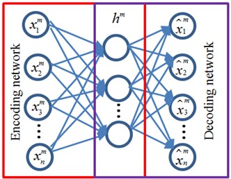
AE (Auto-encoder) is a non-supervised three-layer neural network [23], and it is divided into encoding network and decoding network, as shown in Fig. 1. Input data and output objective are the same for AE. Though the encoding network, input data of high-dimensional space is converted into encoding vectors of low-dimensional space. By the decoding network, the encoding vectors of low-dimensional space are reconstructed into the original input data. Input signals can be reconstructed in the output layer, so that the encoding vector becomes a feature expression of input data.
A no-label mechanical health condition sample set is given. The encoding network converts each training sample into an encoding vector through an encoding function :
where: is an activation function of the encoding network. is a parameter set of the encoding network and satisfies . The encoding vector is inversely converted into a reconstruction expression of by the decoding function :
where: is the activation function of decoding network. is the parameter set of decoding network and satisfies . AE completes training of the whole network by minimizing the reconstruction error between and :
If the encoding vector can reconstruct very well, we can consider that it has reserved most information contained in the training sample data. However, only reserving the information of is not enough to make AE obtain a useful feature expression because mechanical equipment is located in a complicated environment where the sample data can be interfered easily. In addition, due to the change of working condition caused by complicated tasks, sample features will fluctuate under the same health condition. Therefore, it is necessary to restrain AE to a certain extent in order to make it learn a robust feature expression. DAE [24] solved this problem through reconstructing sample data containing noises. Its ideas are as follows: An encoding network adds noises containing certain statistic features into sample data and then encodes samples, so that DAE can learn features with higher robustness from the noise contained samples, and sensitivity of DAE to tiny random disturbance can be reduced.
Firstly, random noises are added into the sample according to distribution [23] in order to convert it into a sample containing noise as follows:
where is random hidden noise. Then, DAE training is completed through optimizing the following objective function:
DAE is encoded and reconstructed by adding noises, and can effectively reduce influences brought by mechanical changes, environmental noises and other random factors on the extracted health condition information to improve robustness of feature expression.
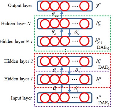
The core of pre-training algorithm for DNN is to stack multiple DAE layer by layer to form a hidden layer structure through a non-supervised method, as shown in Fig. 2. Firstly, the sample is used to train DAE1, and is encoded into the following form:
where: is a parameter of DAE1. can be reconstructed into an input sample, so that major information of can be obtained. Then, is used to train the sample DEA2, and the input is encoded into . This step is repeated until DAEN training is completed, and the input is finally encoded into the following:
During the pre-trainings, multiple DAE are connected mutually to compose a hidden layer structure and realize extraction of fault signals [26]. After completing the pre-training, in order to monitor health conditions of the mechanical equipment, output layers with a classification function are added, and BP algorithm is used to realize minor adjustment of DNN parameters. The output of DNN can be expressed as follows:
where: is a parameter of the output layer. The health condition of is set to be . DNN completes the minor adjustment by minimizing :
Fig. 2Pre-training of DNN
3. Methods of mechanical fault diagnosis
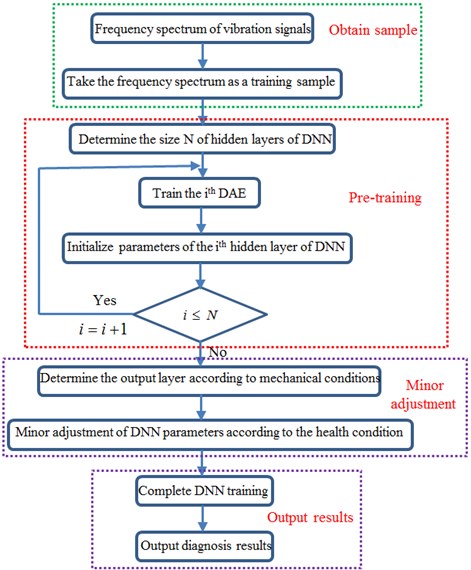
Processes of the method are shown in Fig. 3: firstly, frequency domain signals of the mechanical equipment are obtained, and the frequency spectrum is taken as the training sample; secondly, the size N of hidden layers of DNN is determined and the whole DAE is trained layer by layer in a non-supervised method. The hidden layer output of each DAE is taken as the input of next layer of DAE until the training of the whole DAE is completed; then, output layers are added, DNN parameters are treated by minor adjustment according to heath condition types of the sample, so that DNN training is completed; finally, DNN is used for monitoring and diagnosis of mechanical equipment health conditions.
Fig. 3Flow diagram of fault diagnosis using deep learning
4. Fault diagnosis of standard bearing system
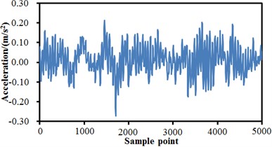
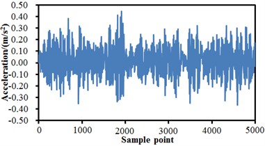
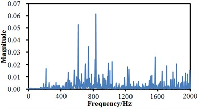
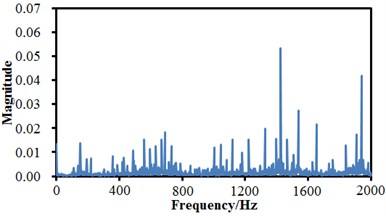
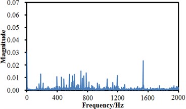
A fault simulation platform of Spectrums Quest Company was adopted as the experimental device. The experimented bearing was a Rexnord deep groove ball bearing, the bearing to be detected supported the rotation shaft of a motor; a single-point damage was processed to the bearing through spark working, with the damage diameter of 0.254 mm; an acceleration sensor was placed on a bearing of the motor and the right side respectively, and the sensors were used to collect vibration acceleration signals of the bearing with fault. The vibration signals were collected by a PULSE analyzer of B&K Company with the sampling frequency of 10000 Hz. In the experiment, data collection was conducted to normal state, inner ring fault, rolling element fault and outer ring fault of the rolling bearing respectively. Each fault was collected under the rotation speed of 300 rpm. 10 groups of data were collected under the rotation speed respectively; data collection of each group lasted for 10 s; each data sample contained 100000 data. Fault vibration signals of the rolling bearing were processed by sensors and A/D sampling, so that original signals of the bearing under each fault condition were obtained. Fig. 4 shows time-domain signals of normal state, inner ring fault, outer ring fault and rolling element fault of the rolling bearing. It is shown in the figure that time-domain signals of the rolling bearing were non-steady signals, and frequency-domain signals could not be obtained through FFT (Fast Fourier Transform) because FFT is mainly aimed at steady signals. FRFT (Fractional Fourier Transform) was conducted to time-domain signals, so that frequency-domain signals were obtained. Results are shown in Fig. 5. With the inner ring fault of the rolling bearing as the example, Fig. 4(b) and Fig. 5(b) are time-domain and frequency-domain figures of the inner ring fault; fault feature information could hardly be found from an original fault waveform of the inner ring. Some side frequencies appeared in the spectrogram of the inner ring fault, but features of the inner ring fault were not very obvious, and a feature frequency corresponding to the rolling bearing could not be recognized accurately. Therefore, the paper tries to use the proposed deep neural network for fault diagnosis of the rolling bearing.
Fig. 4Time-domain signals of rolling bearing under 4 states
a) Normal state
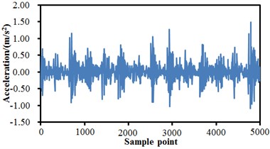
b) Inner ring fault
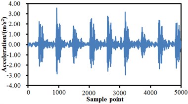
c) Outer ring fault
d) Rolling element fault
Before the fault diagnosis, features of the rolling bearing shall be extracted. Signal features included time-domain features and frequency-domain features. Time-domain statistical analysis of signals refer to estimation and computation of various time-domain feature parameters and indexes of dynamic signals, wherein proper signal dynamic analysis parameters are selected and investigated to judge different types faults. According to existence or inexistence of dimensions, feature values can be divided into dimensional feature values and dimensionless feature values. Sizes of dimensional feature values often vary with conditions such as load, speed and instrument sensitivity, bringing certain difficulty to engineering application. Hence, multiple types of dimensionless indexes are also adopted in mechanical fault diagnosis. Dimensionless parameters are featured by that they are insensitive to changes of mechanical working environment. In other words, they are theoretically unrelated with motion conditions of machines and only rely on the shape of a probability density function. Dimensional feature parameters include peak value, peak-peak value, average amplitude, standard deviation, variance, mean square error, mean square amplitude and root amplitude, etc. Dimensionless feature parameters include skewness degree index, peak value index, waveform index, pulse index, margin index and kurtosis index. Frequency-domain features of signals mainly include gravity frequency and frequency variance. Therefore, feature values of 16 time domains and frequency domains under the different conditions were extracted according to relevant computation formulas, as shown in Table 1, where A is a peak value, B is a peak-peak value, C is an average amplitude, D is a standard deviation, E is a variance, F is a mean square value, G is a root mean square value, H is a root amplitude, I is a skewness degree index, J is a peak value index, K is a waveform index, L is a pulse index, M is a margin index, N is a kurtosis index, O is gravity frequency, and P is a frequency variance.
Fig. 5Frequency-domain signals of rolling bearing under 4 states
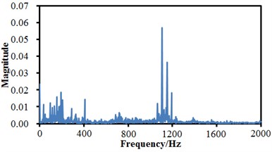
a) Normal state
b) Inner ring fault
c) Outer ring fault
d) Rolling element fault
Table 1Time-domain and frequency-domain feature parameters of 4 faults
Feature parameters | A | B | C | D | E | F | G | H |
Normal state | 0.21 | 0.55 | 0.12 | 0.36 | 0.13 | 0.06 | 0.24 | 0.11 |
Inner ring fault | 1.50 | 2.57 | 0.81 | 1.22 | 1.50 | 1.23 | 1.11 | 0.67 |
Outer ring fault | 3.60 | 6.60 | 1.36 | 3.21 | 10.3 | 1.56 | 1.25 | 1.22 |
Rolling element fault | 0.46 | 0.86 | 0.31 | 0.22 | 0.05 | 0.37 | 0.61 | 0.23 |
Feature parameters | I | J | K | L | M | N | O | P |
Normal state | 0.13 | 2.12 | 0.67 | 1.45 | 2.22 | 3.34 | 501 | 550 |
Inner ring fault | 0.66 | 4.31 | 2.33 | 3.44 | 4.55 | 5.66 | 680 | 655 |
Outer ring fault | 1.11 | 6.60 | 3.45 | 5.61 | 6.73 | 7.23 | 900 | 1100 |
Rolling element fault | 0.34 | 1.89 | 0.45 | 2.33 | 3.46 | 4.21 | 620 | 800 |
Sample data tested were averagely divided into two parts. One part was used to test the samples, and the other part was used to train the samples. It is shown in Table 1 that each fault feature has 16 feature values. Four fault conditions have 64 feature values in total. There are only 4 kinds of faults, so that there are 4 output nodes in the neural network. Other parameter values of the neural network are shown in Table 2.
Table 2Structure parameters of deep neural network
Nodes of input layer | Nodes of output layer | Nodes of hidden layer | Number of nerve cells in hidden layer |
64 | 4 | 3 | 100 |
Non-supervision learning rate | Fine-adjustment learning rate under supervision | Activation function | |
0.1 | 0.01 | Sigmoid function | |
The feature values were taken as the input values input into the neural network so as to conduct fault diagnosis of the rolling bearing. The diagnosis results were compared with results obtained by models such as FANN, PSONN and GANN. Diagnosis accuracy rates are shown in Fig. 6. It is shown in Fig. 6 that 10 experimental results of the deep neural network are obviously better than those of other models. Diagnosis results of different models were processed, as shown in Table 3. It is shown in Table 3 that 10 diagnosis results of the deep neural network were most stable, the diagnosis accuracy rates were very high each time, diagnosis results of other three neural network models fluctuated obviously and had relative large standard deviations, the situation was especially obvious for the GANN model. With the 3rd experiment as the object, error convergence rates of different neural network models under the same experimental conditions were extracted, as shown in Fig. 7.
Fig. 6Comparison of 10 diagnosis results of 4 kinds of neural networks
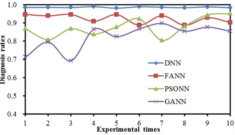
Table 3Comparison of diagnosis results of 4 kinds of neural network models
Method | Maximum | Minimum | Average accuracy rate | Standard deviation / (%) |
DNN | 0.993 | 0.976 | 0.983 | 0.65 |
FANN | 0.945 | 0.871 | 0.924 | 4.38 |
PSONN | 0.912 | 0.807 | 0.878 | 6.94 |
GANN | 0.892 | 0.691 | 0.845 | 12.33 |
During training of a neural network, the number of training iterations reaches 500, or the training error convergence value reaches the critical value of 0.001. Fig. 7 shows comparison of error convergence of 4 kinds of neural networks during one training process. It is shown in Fig. 8 that the DNN model already converged to the critical value of 0.001 when the 48th iteration was conducted. At that moment, training errors of FANN, PSONN and GANN were 0.02, 0.067 and 0.171 respectively, which still had large gaps with the critical error of 0.001. When the iteration number reached 100, the FANN converged to the critical value of 0.001. When the iteration number reached 143, the PSONN converged to the critical error. GANN used GA to improve the neural network, so that optimal points were searched within the global scope for each time of iteration, so that its convergence speed was relatively slow. When the iteration number reached 220, the GANN converged to the critical error. Average statistics was conducted to the iteration process of four kinds of models. Statistic results are shown in Table 4. It is shown in Table 4 that the deep neural network model could converge to the critical value most quickly.
Fig. 7Training process of 4 kinds of neural network models
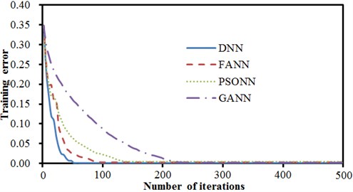
Table 4A comparison of average training results of 4 kinds of neural networks
Network model | Training error | Number of iterations | Time / s |
DNN | 0.001 | 48 | 3.5 |
FANN | 0.001 | 100 | 7.1 |
PSONN | 0.001 | 143 | 5.5 |
GANN | 0.001 | 220 | 52.3 |
5. Fault diagnosis of bogies of the high-speed train based on deep neural networks
It is mentioned in the Introduction that the bogie, as a key component of a high-speed train, often suffers from various failure conditions. Section 4 conducts fault diagnosis of the standard bearing system to highlight that the deep neural network model has a high diagnosis rate and high stability. Therefore, the paper tries to use the deep neural network to conduct systematic and complete diagnosis for failures of bogies.
5.1. Experimental extraction of vibration signals
In the current fault diagnosis of bogies, original data can hardly be obtained by a real experimental device because a failure bogie system will make the high-speed train get out of control and suffer from serious dangers. Therefore, the multi-body dynamics software SIMPACK was often used to simulate a high-speed train bogie to obtain original data. A high-speed train system is a complex mechanical system with multiple degrees of freedom. In order to reflect real performance of the high-speed train as accurately as possible and make the computation and analysis convenient, the following rational hypotheses [27] are made during building a multi-body dynamic model of the high-speed train: 1) structures and parameters of front and rear bogies of the same train are completely the same, and the bogies are symmetric relative to the train center; 2) components such as framework, wheel set and body in the bogies of the train system are taken as rigid bodies, and other types of elastic deformation are not taken into account; 3) only the uneven excitation and disturbance of steel rails are considered, while other types of elastic deformation are not taken into account. Therefore, the high-speed train system can be deemed as a multi-rigid body system which includes 1 train body, 2 bogie frameworks and 4 wheel sets. The train body is connected to the bogie by a secondary suspension. The bogie frameworks are connected to axle boxes of wheel set by a first suspension. The multi-body dynamic model of the high-speed train bogie is established according to the following processes: after obtaining the necessary bogies and technical parameters, the rational hypotheses are used to simplify the train system firstly, where specific steps include definition of basic attributes of each rigid body, definition of three-dimensional geometric shape data of the structure, determination of hinge jointing, applying of force elements and sensors, setting of constraints, and establishment of a topological relation of multi-body elements. Train treads are mainly divided into 4 kinds of types: LMA, LM, S1002 and S1002G. The wheel-track contact relations of four kinds of treads are quite different after they are matched with the Chinese standard steel rail of 60 kg/m (CN60). The research [28] indicates that the train body vibration with the LMA tread had the minimum lateral and vertical accelerations; the S1002G tread had the maximum accelerations, while the lateral accelerations of train body vibration exceeded vertical accelerations. LMA took full account of nonlinearity of wheel-rail contact, creep linearity and non-linear suspension, indicating that the train body with the LMA tread had better stability, and the vertical stability of the train was better than lateral stability. Based on the mentioned hypotheses and analysis, a multi-body dynamic model of the high-speed train system was established, as shown in Fig. 8. Local connection between the bogie and the train body is shown in Fig. 9(a). The multi-body dynamic model of bogies is shown in Fig. 9(b).
Fig. 8Multi-body dynamic model of the high-speed train
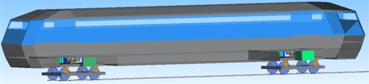
Fig. 9Multi-body dynamic model of bogies and local structures

a) Local structure of connections
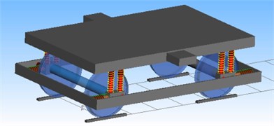
b) Bogies
Many sensors are installed on bogies of the high-speed train. Main parts of bogies include 4 air springs, 4 lateral dampers and 8 anti-yaw dampers. During running of the high speed train, the bogie mainly includes 8 kinds of typical faults: normal condition, failure of lateral damper, failure of anti-yaw damper, failure of air springs, failure of lateral damper + anti-yaw damper, failure of air spring + lateral damper, failure of air spring + anti-yaw damper, failure of lateral damper + anti-yaw damper + air spring. Running speeds under each condition were 200 km/h. The train running was continued for 3.6 min under each condition and sensor data was recorded with the sampling frequency of 250 Hz. 500 sample points were extracted from experimental data per 2 s and taken as one sample. There were 100 samples for each condition. The samples are halved into training samples and testing samples.
In order to simulate real running situations of the high-speed train, it is necessary to input actual track spectrums into the multi-body dynamic model of the high-speed train. Through many experiments, standard track spectrums of the high-speed train were obtained, as shown in Fig. 10. The spectrums were taken as excitation and input into the multi-body dynamic model in Fig. 8. In the published references, the track spectrums of multi-body dynamic model of high-speed train only considered the lateral and vertical directions and failed to take into account the directions with other freedom degrees. The paper not only considers the vertical direction and the lateral direction, but also considers the roll direction and gauge direction, so that simulation of actual running of the high-speed train is relatively better. In addition, it is shown in Fig. 10 that the track spectrums of the high-speed train in different directions had obviously different changing trends and values. The track spectrums of the high-speed train had the maximum in the lateral direction, while it had the minimum in the roll direction.
Fig. 10Track spectrums of the high-speed train
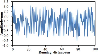
a) Track regularity in lateral direction
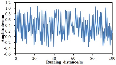
b) Track regularity in vertical direction
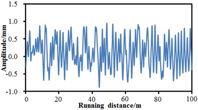
c) Track regularity in gauge direction
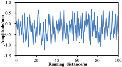
d) Track regularity in roll direction
5.2. Extraction of vibration signals for bogies and experimental validation of the model
The vibration signals of the bogie can be obtained under various conditions after building the mentioned multi-body dynamics model. However, the computational model of the multi-body dynamics model should be necessarily verified through experiments due to its complexity. As shown in Fig. 11.
Fig. 11Test of vibration signal of bogies
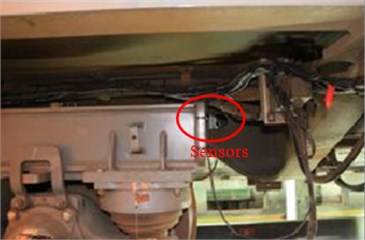
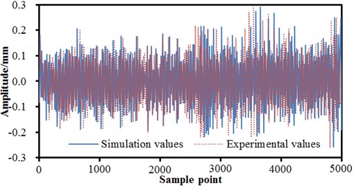
Sensors were mounted on the bogie of the high-speed train which was running at the speed of 200 km/h under the normal condition, so as to test the vibration signal of the bogie and compare it with the computational result of the multi-body dynamics model, which was shown in Fig. 12. It can be seen from the figure that the computational results of the experiment and simulation were basically same except for the slight difference in only individual peak frequencies, indicating that the multi-body dynamics model was reliable and could be used for the subsequent simulation analysis. When fault diagnosis of the bogie was studied, it was not advisable using the experimental test due to the high environmental requirement of the sensor test. Especially in the complex and violent wheel-rail dynamic action, many unpredictable damages would be generated, even causing the inaccurate result of the sensor. In addition, plentiful manpower and financial resources would be spent during the installation of sensors in different parts, and abundant capital input was required for the maintenance of the sensor devices. Therefore, the verified multi-body dynamics model would be taken as the basis in the paper for the subsequent research of the bogie fault of the high-speed train.
Fig. 12Experiment and simulation comparison of vibration signals under normal conditions
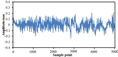
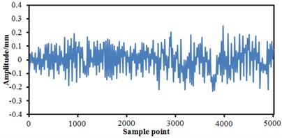
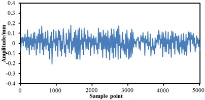
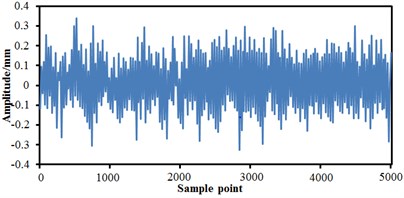
Based on the multi-body dynamic model, multi-mixed failure conditions of bogies can be simulated by setting some related parameters of the model. Fig. 13 and Fig. 15 show the time-domain vibration amplitudes of bogies under a single failure condition and a mixed failure condition. It is shown in Fig. 13 that the time-domain vibration amplitudes of bogies changed in a similar way under the normal condition and air spring failure.
Fig. 13Failure of a single condition for bogies in time domain
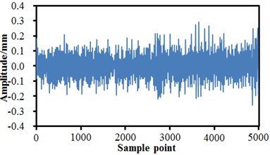
a) Normal state
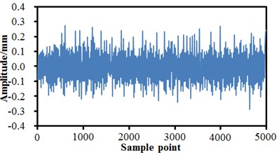
b) Failure of air springs
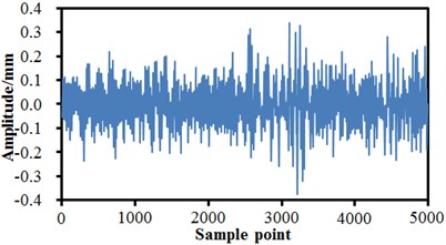
c) Failure of Anti-yaw damper
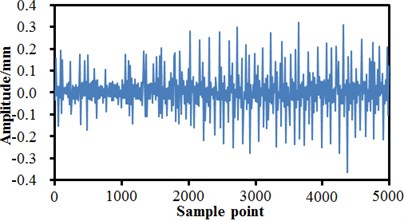
d) Failure of lateral damper
When the anti-yaw damper failed and the lateral damper failed, changing trends of the vibration amplitudes were obviously different. Under the normal state, the maximum time-domain vibration amplitude of the high-speed train was 0.27 mm and the minimum value was –0.26 mm, and the vibration curve did not have a lot of obvious peak values. When the air springs failed, the maximum vibration amplitude was 0.26 mm and the minimum value was –0.3 mm. When the anti-yaw damper failed, the maximum vibration amplitude was 0.34 mm and the minimum value was –0.39 mm. When the lateral damper failed, the maximum vibration amplitude was 0.32 mm, the minimum value was –0.38 mm, and a lot of obvious peak values presented on the whole vibration curve. Fractional Fourier transform was conducted to vibration acceleration signals, so that frequency-domain signals of vibration amplitudes could be obtained, as shown in Fig. 14. It is shown in the figure that the vibration amplitudes were very small or even approached 0 when the analyzed frequency exceeded 80 Hz. In addition, it is shown in Fig. 14(a) and Fig. 14(b) that under the normal state and the failure of air springs, the spectrums of vibration amplitudes were very similar and showed an obvious peak value around 60 Hz. The peak value of normal state was 12 mm, and the peak value of air springs was 14 mm. When the anti-yaw damper failed, the frequency spectrum amplitudes of the high-speed train obviously exceeded those of other three kinds of conditions. The maximum vibration amplitude was 22.1 mm under the corresponding frequency of 2.5 Hz. When the lateral damper failed, the vibration amplitudes of the high-speed train were the minimum on the whole frequency spectrum. There were many obvious peak values on the vibration curve, where the maximum peak value was 9.5 mm under the corresponding frequency of 2.5 Hz. The analyzed results indicate that the failure of lateral damper could be determined just according to the frequency spectrum of vibration amplitudes.
Fig. 14Failure of a single condition for bogies in frequency domain
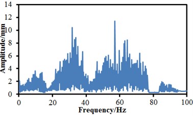
a) Normal state
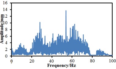
b) Failure of air springs
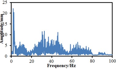
c) Failure of Anti-yaw damper
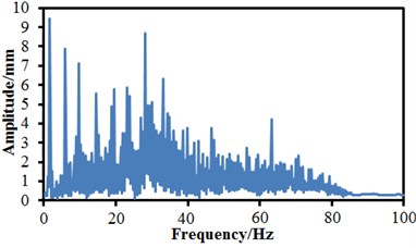
d) Failure of lateral damper
As shown in the above, vibration curves of bogies are only under single condition. Parameters of bogies were set, and vibration features of bogies under the mixed failure condition were extracted, as shown in Fig. 15. Fig. 15(a) shows the condition of failure of lateral damper and anti-yaw damper. It is shown in the figure that the failure of two mixed conditions was not equal to superposition of two single conditions.
When the failure of two kinds of conditions takes place, more peaks and valleys are on the vibration curve, where the maximum and minimum vibration amplitudes are 0.2 mm and –0.2 mm, respectively. Fig. 15(b) shows the condition of failure of lateral damper and air springs. It is thus clear that when two failures take place at the same time, vibrations of the high-speed train are more serious than that generated when the single failure of lateral damper takes place, but it is weaker than that generated when the single failure of air springs takes place. Maximum and minimum of the vibration are 0.28 mm and –0.22 mm, respectively. Fig. 15(c) shows the condition of failures of anti-yaw damper and air springs. It is thus clear that when two types of failures take place at the same time, the vibration curve is relatively serious at the earlier stage of sampling, but it is obviously weaker at the later stage. Fig. 15(d) shows condition when three faults take place at the same time. It is thus clear that a lot of amplitudes and valleys are on the vibration curves, and the vibration became more serious than that under any single failure or two mixed failures, and the maximum and minimum vibration amplitudes are 0.34 and –0.35, respectively.
Fig. 15Failures of mixed conditions for bogies
a) Failures of lateral damper and anti-yaw damper
b) Failures of lateral damper and air springs
c) Failures of anti-yaw damper and air springs
d) Failures of lateral damper, anti-yaw damper and air springs
5.3. Fault diagnosis
Faults of bogies could not be diagnosed according to time-domain and frequency-domain results of vibration amplitudes. Therefore, it is necessary to recognize faults of bogies by an intelligent diagnosis method. Section 4 points out that the deep neural network can obtain a higher diagnosis accuracy rate. Therefore, the paper uses the deep neural network to recognize faults of bogies. During fault diagnosis, the deep neural network shall take time-domain and frequency-domain features of vibration signals as the input. According to relevant computation formulas, feature values of 16 time domains and frequency domains under different conditions were extracted, as shown in Table 5.
Where A is a peak value, B is a peak-peak value, C is an average amplitude, D is a standard deviation, E is a variance, F is a mean square value, G is a root mean square value, H is a root amplitude, I is a skewness degree index, J is a peak value index, K is a waveform index, L is a pulse index, M is a margin index, N is a kurtosis index, O is gravity frequency, and P is a frequency variance. The bogies have 8 working conditions, so that there are 128 nodes in the input layer, and 8 nodes in the output layer. Other relevant parameters are shown in Table 6. The feature values were taken as the input values which were input into the neural network, so that fault diagnosis of bogies could be conducted. The diagnosis results were compared with results obtained by models such as FANN, PSONN and GANN. Diagnosis accuracy rates are shown in Fig. 16. It is shown in Fig. 16 that 10 experimental results of the deep neural network were obviously better than those of other models. Diagnosis results of different models were processed, as shown in Table 7. It is shown in Table 7 that the 10 diagnosis results of the deep neural network were the most stable. The diagnosis accuracy rate was very high each time. Diagnosis results of the other three kinds of neural network models fluctuated obviously with relatively large standard deviations, while the situation was especially obvious for the GANN model. With the 2nd experiment as the object, error convergence speeds of different neural network models under the same experimental conditions were extracted, as shown in Fig. 17.
Table 5Time-domain and frequency-domain feature parameters of bogies under 8 kinds of conditions
Feature parameters | A | B | C | D | E | F | G | H |
Normal state | 0.30 | 0.59 | 0.17 | 0.39 | 0.15 | 0.22 | 0.47 | 0.23 |
Failure of air springs | 0.28 | 0.58 | 0.15 | 0.51 | 0.26 | 0.43 | 0.66 | 0.46 |
Failure of Anti-yaw damper | 0.33 | 0.71 | 0.19 | 1.21 | 1.46 | 0.12 | 0.35 | 0.15 |
Failure of lateral damper | 0.32 | 0.69 | 0.14 | 2.22 | 4.93 | 0.10 | 0.32 | 0.11 |
Failures of lateral and anti-yaw damper | 0.21 | 0.45 | 0.11 | 0.99 | 0.98 | 0.08 | 0.28 | 0.10 |
Failures of lateral damper and air springs | 0.29 | 0.53 | 0.16 | 0.67 | 0.45 | 0.14 | 0.37 | 0.21 |
Failures of anti-yaw damper and air springs | 0.18 | 0.39 | 0.10 | 0.88 | 0.77 | 0.56 | 0.75 | 0.61 |
Failures of lateral, anti-yaw damper and springs | 0.35 | 0.67 | 0.21 | 0.32 | 0.10 | 0.23 | 0.48 | 0.26 |
Feature parameters | I | J | K | L | M | N | O | P |
Normal state | 0.87 | 0.43 | 0.55 | 1.26 | 1.65 | 1.34 | 25 | 650 |
Failure of air springs | 0.99 | 0.56 | 1.10 | 1.77 | 2.01 | 1.67 | 36 | 732 |
Failure of Anti-yaw damper | 1.21 | 0.71 | 1.34 | 2.32 | 2.78 | 2.13 | 18 | 611 |
Failure of lateral damper | 1.13 | 0.88 | 1.22 | 1.81 | 2.33 | 1.69 | 32 | 721 |
Failures of lateral and anti-yaw damper | 0.67 | 0.56 | 0.78 | 1.05 | 1.53 | 1.00 | 26 | 635 |
Failures of lateral damper and air springs | 0.77 | 0.68 | 0.88 | 1.15 | 1.60 | 1.21 | 34 | 725 |
Failures of anti-yaw damper and air springs | 0.89 | 0.83 | 1.01 | 1.44 | 1.89 | 1.32 | 27 | 640 |
Failures of lateral, anti-yaw damper and air springs | 1.23 | 1.11 | 1.56 | 2.66 | 3.22 | 2.41 | 37 | 755 |
Table 6Structural parameters of the deep neural network
Nodes of input layer | Nodes of output layer | Nodes of hidden layer | Number of nerve cells in hidden layer |
128 | 8 | 6 | 200 |
Non-supervision learning rate | Fine-adjustment learning rate under supervision | Activation function | |
0.1 | 0.01 | Sigmoid function | |
Fig. 16Comparisons of 10 diagnosis results of 4 kinds of neural networks
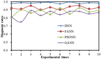
Fig. 17Training process of 4 kinds of neural network models
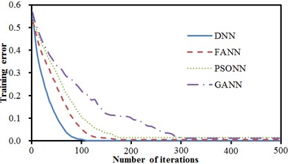
During training of a neural network, the number of training iterations reaches 500, or the training error convergence value reaches the critical value of 0.001. Fig. 17 shows comparisons of error convergence of 4 kinds of neural networks during one training process. It is shown in Fig. 17 that the DNN model already converged to the critical value of 0.001 when the 110th iteration was conducted. At that moment, training errors of FANN, PSONN and GANN were 0.03, 0.095 and 0.211 respectively, which still had large gaps with the critical error of 0.001. When the iteration number reached 190, the FANN converged to the critical value of 0.001. When the iteration number reached 500, the PSONN still could not converge to the critical error, and the final error was 0.008. GANN used GA to improve the neural network, so that optimal points were searched within the global range for each time of iterations, so that its convergence speed was relatively slow. When the iteration number reached 500, the GANN did not converge to the critical error, and only converge to 0.013. Average statistics was conducted to the iteration process of four kinds of models. Statistic results are shown in Table 8. It is shown in Table 8 that the deep neural network model could converge to the critical value most quickly.
Table 7Comparisons of diagnosis results of 4 kinds of neural networks
Method | Maximum | Minimum | Average accuracy rate | Standard deviation / (%) |
DNN | 0.997 | 0.973 | 0.983 | 0.71 |
FANN | 0.950 | 0.901 | 0.924 | 3.25 |
PSONN | 0.925 | 0.805 | 0.878 | 6.77 |
GANN | 0.891 | 0.753 | 0.849 | 10.33 |
Table 8A comparison of average training results of 4 kinds of neural networks
Network model | Training error | Number of iterations | Time / s |
DNN | 0.001 | 110 | 5.4 |
FANN | 0.001 | 190 | 10.2 |
PSONN | 0.008 | 500 | 21.5 |
GANN | 0.013 | 500 | 67.3 |
Fig. 18Relations between diagnosis accuracy and running speed
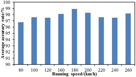
The high-speed train was running at the speed of 200 km/h in the above research. However, high-speed trains were running at many different speeds. Therefore, the deep neural network method was extended for the bogie fault diagnosis under various speeds. Limited by the requirements of vibration and noise, high-speed trains were usually operated at the speed of 80 km/h-260 km/h. The speed step was chosen as 20 km/h to study the bogie fault diagnosis, and the corresponding speed would be 80 km/h, 100 km/h, 120 km/h, 140 km/h, 160 km/h, 180 km/h, 200 km/h, 220 km/h, 240 km/h and 260 km/h, respectively. The diagnostic accuracy of various speeds obtained using the proposed deep neural network was shown in Fig. 18. It could be seen from the figure that the minimum diagnostic accuracy was 96.7 % and the running speed of the high-speed train was 80 km/h. The maximum diagnostic accuracy was 98.9 % with the corresponding running speed of 180 km/h. Different diagnostic accuracies could be caused under different running speeds because the vibration signals of the bogie sensor were different at different speeds, and the computational fault features using the original vibration signal were also different. Finally, the diagnostic accuracy of the deep neural network was different. In the future, the correlation analysis of the sensors arranged in the bogie would be considered in order to obtain the bogie fault features of the high-speed train as many as possible, thus improving the diagnostic accuracy.
6. Conclusions
Based on the previous researches, the paper proposes a deep neural network method to make systematic and complete diagnosis of bogie faults. Firstly, a deep neural network was used to diagnose standard bearing system, and the results were compared with those obtained by traditional neural networks such as FANN, PSONN and GANN. Results show that the deep neural network not only can obtain a high diagnosis accuracy rate and high stability, but it is also the least time-consuming during the whole diagnosis process. Then, a relatively complete multi-body dynamic model of the high-speed train was established, and vibration data of the bogie under the single failure condition and the mixed failure condition were extracted. The deep neural network was used to diagnose 8 kinds of conditions of the bogie systematically. The fault diagnosis was repeated for 10 times. Results obtained for the 10 times indicate obvious advantages of the deep neural network which could obtain the average diagnosis rate of 98.3 % and had the diagnosis standard deviation of 0.71. Finally, training process of one fault diagnosis was extracted. Results show that the deep neural network could converge to a critical value at the quickest speed. All the analysis results indicate that the deep neural network has irreplaceable advantages in intelligent diagnosis of bogies.
References
-
Hayashi Y., Tsunashima H., Marumo Y. Fault detection of railway vehicle suspension systems using multiple-model approach. Journal of Mechanical Systems for Transportation and Logistics, Vol. 1, Issue 1, 2008, p. 88-99.
-
Tsunashima H., Hayashi Y., Mori H., et al. Condition monitoring and fault detection of railway vehicle suspension using multiple-model approach. IFAC Proceedings Volumes, Vol. 41, Issue 2, 2008, p. 8299-8304.
-
Chen T. F., Huang C. L., Fan X. P. Fault diagnosis method for locomotive bogies based on wavelet analysis. China Railway Science, Vol. 26, Issue 4, 2005, p. 89-92.
-
Huang C. L., Fan X. P., Chen C. Y., et al. Fault diagnosis method of locomotive driven gear based on envelopment analysis of wavelet coefficients extraction and DCT. Journal of the China Railway Society, Vol. 30, Issue 2, 2008, p. 98-102.
-
Ding X. W., Liu B., Liu J. Z., et al. Fault diagnosis of freight car rolling element bearings with adaptive short-time Fourier transform. China Railway Science, Vol. 25, Issue 6, 2005, p. 24-27.
-
Chen L., Zi Y. Y., Cheng W., et al. EEMD-1.5 dimension spectrum applied to locomotive gear fault diagnosis. Proceedings of International Conference on Measuring Technology and Mechatronics Automation, Vol. 1, 2009, p. 622-625.
-
Lei Y. G., He Z. J., Zi Y. Y. Application of a novel hybrid intelligent method to compound fault diagnosis of locomotive roller bearings. Journal of Vibration and Acoustics, Transactions of the ASME, Vol. 130, 2008, p. 3-34501.
-
Lei Y. G., He Z. J., Zi Y. Y. EEMD method and WNN for fault diagnosis of locomotive roller bearings. Expert Systems with Applications, Vol. 38, Issue 6, 2011, p. 7334-7341.
-
Jousselme A. L., Liu C. S., Grenier D. Measuring ambiguity in the evidence theory. IEEE Transactions on Systems, Man, and Cybernetics-TSME, Part A, Vol. 36, Issue 5, 2006, p. 890-903.
-
Garcia C. R., Andreas L. Comparison of collision avoidance system and applicability to rail transport. Proceedings of the 7th International Conference on Intelligent Transport Systems, Sophia Antipolis, Francs, 2007.
-
Garcia C. R., Lehner A., Strang T. Channel model for train to train communication using the 400 MHz band. Proceedings of the 67th Vehicular Technology Conference. Singapore, 2008.
-
Ngigi R. W., Pislaru C., Ball A., et al. Modern techniques for condition monitoring of railway vehicle dynamics. Journal of Physics: Conference Series, Vol. 364, 2012, p. 1-12016.
-
Chen B., Zhang Z., Sun C., et al. Fault feature extraction of gearbox by using overcomplete rational dilation discrete wavelet transform on signals measured from vibration sensors. Mechanical Systems and Signal Processing, Vol. 33, 2012, p. 275-298.
-
Hinton G. E., Salakhutdinov R. Reducing the dimensionality of data with neural networks. Science, Vol. 313, Issue 7, 2006, p. 504-507.
-
Hinton G. E., Osindero S., Whye Y. A fast learning algorithm for deep belief nets. Neural Computation, Vol. 18, 2006, p. 1527-1554.
-
Dahl G. E., Yu D., Deng L., et al. Context-dependent pre-trained deep neural networks for large-vocabulary speech recognition. IEEE Transactions on Audio, Speech, and Language Processing, Vol. 20, Issue 1, 2012, p. 30-42.
-
Tang J., Deng C., Huang G. B., et al. Compressed-domain ship detection on space borne optical image using deep neural network and extreme learning machine. IEEE Transactions on Geoscience and Remote Sensing, Vol. 53, Issue 3, 2015, p. 1174-1185.
-
Vincent P., Larochelle H., Lajoie I., et al. Stacked denoising auto encoders: Learning useful representations in a deep network with a local denoising criterion. Journal of Machine Learning Research, Vol. 11, 2010, p. 3371-3408.
-
Pang R., Yu Z. B., Xiong W. Y., Li H. Faults recognition of high-speed train bogie on deep learning. Journal of Railway Science and Engineering, Vol. 12, Issue 6, 2015, p. 1283-1288.
-
Xie J. P., Li T., Yang Y., et al. Learning features from high speed train vibration signals with deep belief networks. International Joint Conference on Neural Networks (IJCNN), 2014, p. 2205-2210.
-
Guo C., Yang Y., Pan H., et al. Fault analysis of High Speed Train with DBN hierarchical ensemble. International Joint Conference on Neural Networks (IJCNN), 2016, p. 2552-2559.
-
Yin J., Zhao W. Fault diagnosis network design for vehicle on-board equipments of high-speed railway: a deep learning approach. Engineering Applications of Artificial Intelligence, Vol. 56, 2016, p. 250-259.
-
Bengio Y. Learning deep architectures for AI. Foundations and Trends in Machine Learning, Vol. 2, Issue 1, 2009, p. 1-127.
-
Erhan D., Bengio Y., Courville A. Why does unsupervised pre-training help deep learning? The Journal of Machine Learning Research, Vol. 11, 2010, p. 625-660.
-
Vincent P., Larochelle H., Lajoie I., et al. Stacked denoising auto encoders: Learning useful representations in a deep network with a local denoising criterion. The Journal of Machine Learning Research, Vol. 11, 2010, p. 3371-3408.
-
Silver D., Huang A., Maddison C. J., et al. Mastering the game of Go with deep neural networks and tree search. Nature, Vol. 529, Issue 7587, 2016, p. 484-489.
-
Zolotas A. C., Pearson J. T., Goodall R. M. Modelling requirements for the design of active stability control strategies for a high speed bogie. Multibody System Dynamics, Vol. 15, Issue 1, 2006, p. 51-56.
-
Zhang M., Zhang L., Luo Y. P., Dong D. C. Simpack modeling and analysis of the high-speed EMU bogie dynamic performance. China Metros, Vol. 10, 2015, p. 36-41.
Cited by
About this article

This work is supported by Dongguan Social Science and Technology Development Project and Science Research Project of Guangdong University of Science and Technology.
