Abstract
Vibration-based analysis is the most commonly used technique to monitor the condition of gearboxes. Accurate classification of these vibration signals collected from gearbox is helpful for the gearbox fault diagnosis. In recent years, deep neural networks are becoming a promising tool for fault characteristic mining and intelligent diagnosis of rotating machinery with massive data. In this paper, a study of deep neural networks for fault diagnosis in gearbox is presented. Four classic deep neural networks (Auto-encoders, Restricted Boltzmann Machines, Deep Boltzmann Machines and Deep Belief Networks) are employed as the classifier to classify and identify the fault conditions of gearbox. To sufficiently validate the deep neural networks diagnosis system is highly effective and reliable, herein three types of data sets based on the health condition of two rotating mechanical systems are prepared and tested. Each signal obtained includes the information of several basic gear or bearing faults. Totally 62 data sets are used to test and train the proposed gearbox diagnosis systems. Corresponding to each vibration signal, 256 features from both time and frequency domain are selected as input parameters for deep neural networks. The accuracy achieved indicates that the presented deep neural networks are highly reliable and effective in fault diagnosis of gearbox.
1. Introduction
Industrial environments have constantly increasing requirements for the continuous working of transmission machines. That is why new proposals for building fault diagnostic systems with low complexity and adequate accuracy are highly valuable [1]. As one of the core components in rotary machinery, gearbox is widely employed to deliver torque or provide speed conversions from rotating power sources to other devices [2]. Identifying gearbox damage categories, especially early faults and combined faults, is an effective way to avoid fatal breakdowns of machines and prevent loss of production and human casualties. The vibration signals during the run-up and run-down periods of a gearbox contain a wealth of condition information [3]. Vibration-based analysis is the most commonly used technique to monitor the condition of gearboxes.
In gear fault diagnosis, several analysis techniques have been used, such as wavelet transform [4, 5], group sparse representation [6], multiscale clustered grey infogram [3], and generalized synchrosqueezing transform [7]. The availability of an important number of condition parameters that are extracted from gearbox signals, such as vibration signals, has motivated the use of machine learning-based fault diagnosis, where common approaches use support vector machine [8, 9], neural networks (NN) [10-13] and their related models, because of the simplicity for developing industrial applications.
The SVM family received good results in comparison with the peer classifiers [14]. In [13], a comparison study was conducted on three types of neural networks: feedforward back-propagation (FFBP) artificial neural network, functional link network (FLN) and learn vector quantization (LVQ). The study achieved good results with FFBP for the classification of three faults at different rotation frequencies. However, as Y. Bengio reported in [15, 16], the gradient-based training of supervised multi-layer neural networks (starting from random initialization) gets easily stuck in “apparent local minima or plateaus”, which is to restrict its application in more complex gearbox fault diagnosis.
In recent years, deep neural networks are becoming a promising tool for fault characteristic mining and intelligent diagnosis of rotating machinery with massive data [17]. Since 2006, deep learning networks such as Restricted Boltzmann Machine (RBM) [18], Deep Belief Networks (DBN) [19] have been applied with success in classification tasks and other fields such as in regression, dimensionality reduction, and modeling textures [20]. Some reports showed that the deep learning techniques have been applied for the fault diagnosis with commonly one modality feature. Tran et al. [21] suggested a DBN-based application to diagnose reciprocating compressor valves. Tamilselvan and Wang [22] employed the deep belief learning for health state classification of iris dataset, wine dataset, Wisconsin breast cancer diagnosis dataset, and Escherichia coli dataset. C. Li et al [23] proposed multimodal deep support vector classification for gearbox fault diagnosis, where Gaussian-Bernoulli deep Boltzmann machines (GDBMs) were used to extract the feature of the vibration and acoustic signal in time, frequency and wavelet modalities, respectively; and then the extracted features are integrated for fault diagnosis using GDBMs. Li’s research [23] indicated that Gaussian-Bernoulli deep Boltzmann machine is effective for the gearbox fault diagnosis. We have presented a multi-layer neural network (MLNN) for gearbox fault diagnosis (MLNNDBN) [24], where the weights of deep belief network are used to initialize the weights of the constructed MLNN. Experiment results showed MLNNDBN was an effective fault diagnosis approach of gearbox. However, data sets were only collected from an experimental rig, which only included 12 kinds of condition parameters.
There are growing demands for condition-based monitoring of gearboxes, and techniques to improve the reliability, effectiveness and accuracy for fault diagnosis are considered valuable contributions [25]. In this work, basing on the time-domain and frequency-domain features extracted from vibration signal, we evaluated the performance of four classical deep neural networks (Auto-encoders, Restricted Boltzmann Machines, Deep Boltzmann Machines and Deep Belief Networks) for gearbox fault diagnosis. In the existing researches of intelligent gearbox fault diagnosis systems, their experimental data sets were usually obtained from a simple experimental rig, where a signal only corresponds to one type of gear or bearing fault, and one data set only involves the classification of several fault condition patterns. As a result, it is insufficient to validate the generalization of an intelligent diagnosis system. To ensure that the proposed diagnosis systems are highly effective and reliable in fault diagnosis of industrial reciprocating machinery, three types of data sets based on the health condition of two rotating mechanical systems are prepared and tested in our study. Each signal obtained includes the information of several basic gear or bearing faults. Totally 62 data sets are used to test and train the proposed gearbox diagnosis systems.
The rest of this paper is constructed as follows. Section 2 introduces the adoptive methodologies including Auto-encoders, Restricted Boltzmann Machines, Deep Boltzmann Machines and Deep Belief Networks; Section 3 covers feature representation of vibration signals; Section 4 presents the implementation of the classifier based on deep neural networks; Section 5 is an introduction of experimental setup; Results and discussion are presented in Section 6; The conclusions of this work are given at the end.
2. Deep neural networks
The essence of deep neural networks (DNN) is to build neural network by imitating the hierarchical structure of human visual mechanism and brain to analyze and learn things. By establishing machine learning model with multiple hidden layers and using a sea of training data, deep neural network is to learn more useful features so as to improve the accuracy of classification and prediction. Compared with traditional shallow learning, the distinctiveness of deep neural network lies in that: (1) it emphasizes the depth of model structure which usually has hidden layer nodes of five layers, six layers, or even over ten layers; (2) it explicitly highlights the importance of feature learning, that is, to transform the feature expression of the sample from the original space to a new feature space via feature shifts layer by layer, thereby making classification or predictions easier. Compared with the method of regular artificial configuration, using big data to learn feature may better depict the abundant inner information of data.
The training mechanism of deep neural network includes two stages: the first stage is to use bottom-up unsupervised learning. This process can be regarded as a process of feature learning. The second stage is to use top-down supervised learning, which usually applies the gradient descent method to fine-tune the whole network parameters. The fundamental steps are given as follows:
Step 1: Build neurons layer by layer. For any two neighboring layers, suppose the input layer is the lower layer while the other layer is the upper layer. The connection weights between layers include cognitive weights upward from the lower layer to the upper one and the generative weights from the upper layer to the lower one. The cognitive process upward is actually the encoding stage (Encoder), which is to extract feature (Code) from the bottom to the top. The reconstruction downward is actually the decoding stage (Decoder), which is to rebuild information for the abstract expression and the generative weights.
Step 2: Adjust parameters layer by layer based on the wake-sleep algorithm. This process is for feature learning in which the parameters in one layer are adjusted.
Step 3: Apply top-down supervised learning. This step is to add a classifier (such as Logistic Regression, SVM, etc.) at the top encoding layer based on the parameters of each layer acquired through learning of the second step. Then apply gradient descent method to fine-tune the whole network parameters through data-labeled supervised learning.
In the following subsections, four commonly-used deep neural networks, Restricted Boltzmann Machine (RBM), Deep Boltzmann Machine (DBM), Deep Belief Networks (DBN) and Stack Auto-encoders (SAE) will be briefly discussed. For more details, please refer to the relevant literature [18, 19, 26, 27].
2.1. Restricted Boltzmann machine
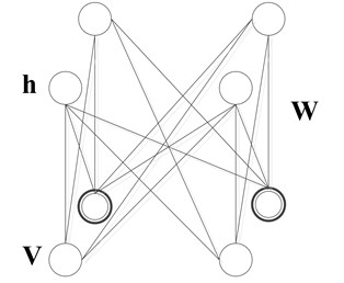
The restricted Boltzmann machine is a generative stochastic artificial neural network with two layers as shown in Fig. 1, which can learn a probability distribution over its set of inputs. The standard RBM has binary-valued hidden and visible units, and consists of a matrix of weights associated with the connection between hidden unit and visible unit. Given these, an energy function of the configuration (, ) is defined as following [18]:
where and denote the visible and the hidden neurons, and stand for their offsets, and is network parameters. To accommodate the real-valued input data, Salakhutdinov et al. [28] proposed Gaussian-Bernoulli RBM (GRBM), where the binary visible neurons can be replaced by the Gaussian ones. The energy function is redefined as the following:
where is the standard deviation associated with Gaussian visible neuron . The statistical parameters for the fault diagnosis are real-valued, so Eq. (2) is selected as the energy function in this paper.
Fig. 1A restricted Boltzmann machine
The probability that the network assigns to every possible pair of a visible and a hidden vector is given via this energy function as the following:
where is called as “partition function” and defined as the sum of over all possible configurations.
The network assigns probability to a visible vector, , is given by summing over all possible hidden vectors:
By adjusting to lower the energy of a training sample and to raise the energy of other samples, the probability that the network assigns to the training sample can be raised, especially those which have low energies and then make a big contribution to the partition function.
A standard approach to estimate the parameters of a statistical model is maximum-likelihood estimation, which maximizes the likelihood by using the training data to train the parameters . The likelihood is defined as:
where represents the set of samples and is the size of . Maximizing the likelihood is the same as maximizing the log-likelihood given by:
Gradient descent method is usually employed to find the maximum likelihood parameters analytically. The derivative of the log probability of a training data with respect to is given by:
Because there are no direct connections between the hidden units in an RBM, it is very easy to calculate the first item of Eq. (7). Given a randomly selected training data (real-valued), , the binary state of each hidden unit, , is set to 1 with probability:
where is a sigmoid function. Similarly, given a hidden vector , is set to 1 with probability:
where expresses normal distribution function.
However, it is much more difficult to get the second item. It can be done by starting at any random state of the visible units and performing alternating Gibbs sampling for a very long time. An iteration of alternating Gibbs sampling consists of updating all of the hidden units in parallel using Eq. (8) followed by updating all of the visible units in parallel using Eq. (9).
The algorithm performs Gibbs sampling and is used inside a gradient descent procedure to compute weight, which is updated as the following [29]:
(1) Take a training sample , compute the probabilities of the hidden units and sample a hidden activation vector from this probability distribution.
(2) Compute the outer product of and and call this the positive gradient.
(3) From , sample a reconstruction of the visible units, then resample the hidden activations from this. (Gibbs sampling step).
(4) Compute the outer product of and and call this the negative gradient.
(5) Update the weight: . is expressed as: the positive gradient minus the negative gradient, the result of which times some learning rate.
The update rule for the biases and is defined analogously.
2.2. Deep Boltzmann machine
A deep Boltzmann machine (DBM) [28] is undirected graphical models with bipartite connections between adjacent layers of hidden units, which is a network of symmetrically coupled stochastic units. Similar to RBMs, this binary-binary DBM can be easily extended to modeling dense real-valued count data. For real-valued cases, Cho et al. [30] proposed a Gaussian-Bernoulli deep Boltzmann machine (GDBM) which used the Gaussian neurons in the visible layer of the DBM. Fig. 2(b) presents a three-hidden-layer DBM, whose energy is defined as Eq. (10), where is the number of hidden layers:
Salakhutdinov et al. [28] introduced a greedy and layer-by-layer pretraining algorithm by learning a stack of modified RBMs for DBM model, where contrastive divergence learning [25] works well and the modified RBM is good at reconstructing its training data. In this modified RBM with tied parameters, the conditional distributions over the hidden and visible states are defined as Eq. (11) and Eq. (12):
where is a sigmoid function. When a stack of more than two RBMs is greedily being trained, the modification only needs to be used for the first and the last RBM in the stack. For all the intermediate RBMs, simply halve their weights in both directions when composing them to form a deep Boltzmann machine. It should be noted that there are two special cases: the last and the first hidden layers for the above equation. For the last hidden layer (i.e., ), we set 0. As for the first hidden layer (i.e., 1), parameters for Eq. (12) should be set as:
Fig. 2DBN&DBM
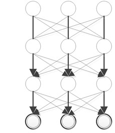
a) Deep belief network
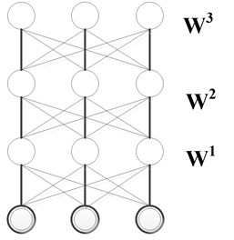
b) Deep Boltzman machine
2.3. Deep belief networks
Deep belief networks (DBNs) [19] can be viewed as another greedy, layer-by-layer unsupervised learning algorithm that consists of learning a stack of RBMs one layer at a time. The top two layers form a restricted
Boltzmann machine which is an undirected graphical model, but the lower layers form a directed generative model (see Fig. 2(a)). The training algorithm for DBNs proceeds as follows. Let be a matrix of inputs, and regarded as a set of feature vectors.
(1) Train a restricted Boltzmann machine on to obtain its weight matrix, , and use this as the weight matrix between the lower two layers of the network.
(2) Transform by the RBM to produce new data .
(3) Repeat this procedure with for the next pair of layers, until the top two layers of the network are reached.
(4) Fine-tune all the parameters of this deep architecture with respect to the supervised criterion.
2.4. Stacked Auto-encoders
The Auto-encoder is trained to encode the input into some representation so that the input can be reconstructed from that representation [29]. Hence the target output of the auto-encoder is the auto-encoder input itself. If there is one linear hidden layer and the mean squared error criterion is used to train the network, then the hidden units learn to project the input in the span of the first principal components of the data. Auto-encoders have been used as building blocks to build and initialize a deep multi-layer neural network [15, 30, 31]. The training procedure is similar to the one for Deep Belief Networks. The principle is exactly the same as the one previously proposed for training DBNs, but auto-encoders instead of RBMs are used as the following [20]:
(1) Train the first layer as an auto-encoder to minimize some forms of reconstruction errors of the raw input.
(2) The outputs of hidden units on the auto-encoder are used as input for another layer, which is also trained to be an auto-encoder.
(3) Iterate as step (2) to initialize the desired number of additional layers.
(4) Take the last hidden layer output as input to a supervised layer and initialize its parameters (either randomly or by supervised training, keeping the rest of the network fixed).
(5) Fine-tune all the parameters of this deep architecture with respect to the supervised criterion. Alternately, unfold all the auto-encoders into a very deep auto-encoder and fine-tune the global reconstruction error, as in [32].
3. Feature representations of vibration signals
In this section, the feature extraction of vibration signal will be introduced. The gearbox condition can be reflected through the information included in different time, frequency and time-frequency domain. The features in frequency and time domain are extracted from the set of signals obtained from the measurements of the vibrations at different speeds and loads, which are used as input parameters for the deep neural network.
3.1. Frequency-domain feature extraction
For a vibration signal of the gearbox, , its spectral representation can be calculated by Eq. (14):
where the “^” stands for the Fourier transform, is the time and is the frequency.
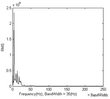
The time domain signal was multiplied by a Hanning window to obtain the FFT spectrum. The spectrum can be divided into multiple bands, and the root mean square value (RMS) for each band keeps track of the energy in the spectrum peaks. RMS value is evaluated with Eq. (15), where is the number of samples of each frequency band:
Fig. 3 and Fig. 4 present the FFT spectrum and its RMS representation of a vibration signal, respectively. It is obvious that the root mean square (RMS) values keep track of the energy in the spectrum peaks. To reduce the number of input data, the spectrum was split in multiple bands and the RMS value of each band is used as feature representation in the spectrum domain.
Fig. 3Original frequency representation
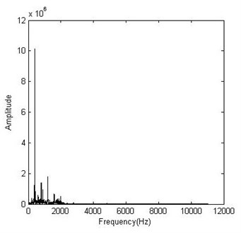
Fig. 4Frequency representation using RMS values
3.2. Time-domain feature extraction
The time-domain signal collected from a gearbox usually changes when damage occurs in a gear or bearing. Both its amplitude and distribution may be different from those of the time-domain signal of a normal gear or bearing. Root mean square value reflects the vibration amplitude and energy in time domain. Standard deviation, skewness and kurtosis may be used to represent time series distribution of the signal in time domain.
Fig. 5Gearbox fault diagnosis based on deep neural networks
Four time-domain features, namely, standard deviation, mean value, skewness and kurtosis are calculated. They are defined as follows.
(1) Mean value:
(2) Standard deviation:
(3) Skewness:
(4) Kurtosis:
To sum up, the vector of the features of the preprocessed signal is formed as follows: RMS values, standard deviation, skewness, kurtosis, rotation frequency and applied load measurements, which are used as input parameters for the deep neural networks. In this paper, is set to 251.
4. DNN-based classifier
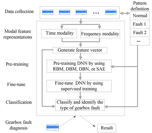
In this section, the implementation of the classifier based on DNN will be introduced. Fig. 5 presents the outline of DNN-based gearbox fault diagnosis.
In the pre-training stage, RBM, DBM, DBN or SAE (see their detail implementation and parameters settings in [18, 19, 26, 27]) are employed as pre-training strategies of DNN for gearbox fault diagnosis respectively. At the second stage, the parameters of the whole network is fine-tuned by using supervised training. The training procedure is shown in Fig. 6, which presents the pseudo-code of DNN-based classifier followed in the processing of the signal. A batch training strategy is used to train the neural network, where the weights of nets are shared by a batch of training samples with mini batches of size.
5. Experimental setup
To validate the effectiveness of the proposed method for fault diagnosis, we constructed three kinds of vibration signal data sets based on the health condition of two rotating mechanical systems. The experimental set-ups and the procedures are detailed in the following subsections.
5.1. Data set I
The data set I of vibration signal includes different basic fault patterns as defined in Table 1 for the gearbox diagnosis experiments. 11 patterns with 3 different load conditions (300, 600, and 900 rpm) and 3 different input speeds (zero, small, and great) were applied during the experiments. For each pattern, load and speed condition, we repeated the tests for 5 times. Each time, the vibration signals were collected with 24 durations, each duration covered 0.4096 sec. The sampling frequency for the vibration signals was set for 50 kHz and 10 kHz, respectively.
Fig. 6Pseudo-code of DNN-based classifier
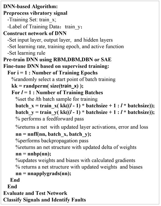
Fig. 7a) Fault simulator setup; b) Internal configuration of the gearbox
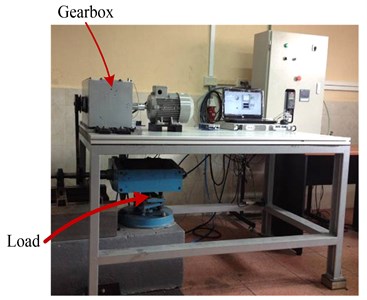
a)
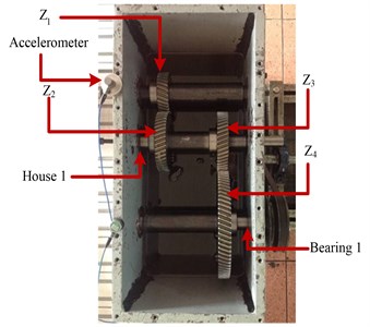
b)
Data set I was obtained from the measurements of a vertically allocated accelerometer in the gearbox fault diagnosis experimental platform shown in Fig. 7. Fig. 7(a) shows the fault simulator setup of the gearbox. A motor (SIEMENS, 3, 2.0 HP) through a coupling is used, whose speed is controlled by a frequency inverter (DANFOSS VLT 1.5 kW). An electromagnetic torque load is used, which is controlled by a torque controller (TDK-Lambda, GEN 100-15-IS510). The vibration signals of the gearbox were collected by an accelerometer (PCB ICP 353C03). Fig. 7(b) shows the internal configuration of the gearbox, which is a two-stage transmission of the gearbox. The parameters of all components on the gearbox are listed here: Input helical gear: 30, modulus = 2.25, impact angle = 20°, and helical angle = 20°; Two intermediate helical gears: 45; and the output gear: 80. The faulty components used in the experiments include gears , , , and , bearing 1 and house 1 are labeled in Fig. 7(b). Based on the above experimental platform of gearbox fault diagnosis, 11880 vibration signals (i.e., [, …, ]) corresponding to 11 condition patterns (i.e., [, , …, ]) have been recorded.
Table 1Condition patterns of the gearbox configuration
Faulty pattern | – | |||||
Faulty component | Gear | Gear | Gear | Gear | Gear | – |
Faulty detail | Worn tooth | Chaffing tooth | Pitting tooth | Worn tooth | Chipped tooth | – |
Faulty photo |  |  |  |  |  | – |
Faulty pattern | B6 | B7 | B8 | B9 | B10 | |
Faulty component | Gear Z4 | Bearing 1 | Bearing 1 | Bearing 1 | House 1 | N/A |
Faulty detail | Root crack tooth | Inner race fault | Outer race fault | Ball fault | Eccentric | N/A |
Faulty photo |  |  |  |  |  | N/A |
5.2. Data set II
In data set I, each vibration signal only includes information of one fault component, which has only a kind of fault. However, there are usually two or more fault components in the real-world rotating mechanical system. In order to evaluate whether the proposed approach is applicable in fault diagnosis of industrial reciprocating machinery, data set II is constructed, where each fault pattern includes two or more basic faults. Firstly, some basic faults are defined in Table 2 and Table 3, which include 11 kinds of basic gear faults and 8 kinds of bear faults, respectively. 12 combined fault patterns are defined in Table 4.
Table 2Nomenclature of gears fault
Designator | Description |
Normal | |
Gear with face wear 0.6 [mm] | |
Gear with face wear 0.3 [mm] | |
Gear with chafing in tooth 40 % | |
Gear with chafing on tooth 100 % | |
Gear with pitting on tooth depth 0.1 [mm], width 0.6 [mm], and large 0.05 [mm] | |
Gear with pitting on teeth | |
Gear with incipient fissure on 5mm teeth to 30 % of profundity and angle of 45° | |
Gear teeth breakage 25 % | |
Gear teeth breakage 60 % | |
Gear teeth breakage 100 % |
Data set II was obtained from the measurements of a vertically accelerometer on another gearbox fault diagnosis experimental platform. Fig. 8 indicates the internal configuration of the gearbox and positions for accelerometers, which is a two-stage transmission of the gearbox with 3 shafts and 4 gears. The parameters of all components on this gearbox are as follows: Input gear: 27, modulus = 2, and of pressure = 20; Two intermediate gears: 53; and the output gear: Z4= 80. The faulty components used in the experiments include gears , , , and , bearing , , , and as labeled in Fig. 8(a). The conditions of the test are described in the Table 5, where 4 different load conditions and 5 different input speeds were applied for each fault pattern during the experiments. For each pattern with different load and speed condition, we repeated tests for 5 times. Each time, the vibration signals were collected with 10 durations, each duration covered 0.4096 sec.
Table 3Nomenclature of bearing fault
Designator | Description |
Normal | |
Bearing with 2 pitting on outer ring | |
Bearing with 4 pitting on outer ring | |
Bearing with 2 pitting on inner ring | |
Bearing with 4 pitting on inner ring | |
Bearing with race on Inner ring | |
Bearing with 2 pitting on ball | |
Bearing with 2 pitting on ball |
Table 4Condition patterns of the experiment
Number of patterns | Basic faults | |||||||
Gear faults | Bear faults | |||||||
Table 5The conditions of the test
Characteristic () | Value |
Sample frequency | 44100 [Hz] (16 bits) |
Sampled time | 10 [s] |
Power | 1000 [W] |
Minimum speed | 700 [RPM] |
Maximum speed | 1600 [RPM] |
Minimum load | 250 [W] |
Maximum load | 750 [W] |
Speeds | 1760, 2120, 2480, 2840, and 3200 [mm/s] |
Loads | 375,500,625, and 750 [W] |
Number of loads per test | 10 |
Type of accelerometer | Uni-axial |
Trademark | ACS |
Model | ACS 3411LN |
Sensibility | 330 [mV/g] |
Based on the above experimental platform for gearbox fault diagnosis, data set II has 12000 vibration signals (i.e., [, …, ]) corresponding to 12 combined condition patterns (i.e., [, , …, ]) to be recorded.
Fig. 8a) Internal configuration of the gearbox; b) Positions for accelerometers
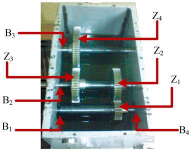
a)
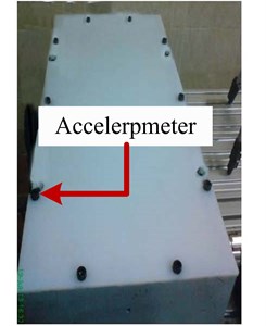
b)
5.3. Data set III
One or two test cases cannot fully reflect the reliability and robustness of an algorithm. Although some classifiers are effective for some special data sets, they get easily stuck in “apparent local minima or plateaus” in some other cases, resulting in a disability to classify fault patterns effectively. To further validate the reliability and robustness of the DNN, a fault condition pattern library has been constructed, which has 55 kinds of condition patterns based on the fundamental patterns described in Table 2 and Table 3. Each condition pattern holds more than one basic gearbox fault.
To challenge the proposed approaches, we have generated a large number of data sets. Each data set includes kinds of condition patterns. Here three kinds of ’s value are considered for these data sets: 12, 20 and 30, respectively. It is obvious that bigger value of means the classification and identification of faults are more difficult. For each size of , 20 different data sets were generated, where each one involves unique combination of condition patterns that are randomly selected from the above mentioned pattern library.
Here each data set is collected from the measurements of a vertically accelerometer on the gearbox fault diagnosis experimental platform shown in Fig. 8, whose test conditions and generating method are the same as that of data set II. Each data set has 12000 vibration signals (i.e., [,…, ]) corresponding to each combination of condition patterns (i.e., [, , …, ]). Here expresses th data set, and [, ,…, ] is a combination randomly selected from the pattern library. 60 different data sets are generated in total to further evaluate the performance of the proposed approaches.
6. Experiment and discussion
In this section, we will evaluate the performance of DBN, DBM,RBM and SAE based on data sets defined in Section 4. Based on feature extracting method, feature representations of each vibration signal are formulated as a vector with 256 dimensions, which includes 251 RMS values, standard deviation, skewness, kurtosis, rotation frequency and applied load measurements. These features are regarded as the input of neural network.
6.1. Parameters tuning
As mentioned above, the training of DNN includes two stages: pre-training and fine-tuning. At the stage of fine-tuning, the DNN is usually treated as a feed-forward neural network (FFNN) by using supervised training. FFNN is also typically used in supervised learning to make a prediction or classification. To evaluate the performance of DNN, a comparison study between FFNN with DNN is presented for gearbox fault diagnosis. The net parameters are set as Table 6-7. Based on different training parameters, five typical FFNNs are defined in Table 8. Four parameters (nn.n, nn.unit, nn.epoch1 and nn.epoch2) are fine-tuned based on data set I and data set II as follows.
Table 6Definition of net parameters
Symbols | Description |
nn | Represent the whole neural network. |
nn.n | The number of layers |
nn.size | A vector of describing net architecture parameters including the number of neuron each layer |
nn.epoch1 | The epochs of pre-training using RBM, DBM, DBN or SAE in the first stage training. |
nn.epoch2 | The epochs of fine-training |
nn.act_func | Activation functions of hidden layer: sigmoid or optimal tanh |
nn.output | Activation functions of output layer: sigmoid, softmax or linear function. |
nn.lRate | Learning rate in the second stage training |
nn.mom | Momentum |
nn.wp | A penalty factor for the deltas of updating weights. |
nn.df | “Dropout” fraction of each hidden unit is randomly omitted |
Table 7Setting of training parameters at the pre-training stage
Parameters | RBM | DBN | DBM | SAE |
nn.act_func | Sigmoid | Sigmoid | Sigmoid | Sigmoid |
nn.lRate | 1 | 1 | 1 | 0.01 |
nn.mom | 0 | 0 | 0 | 0 |
nn.wp | 0.5 | 0.5 | 0.5 | 0.5 |
Table 8Setting of training parameters for FFNN
Classifier | nn.act_func | nn.output | nn.lRate | nn.mom | nn.wp | nn.df |
FFNN Scheme1 | Optimal tanh | Sigmoid | 2 | 0.5 | 0 | 0 |
FFNNScheme2 | Optimal tanh | Sigmoid | 2 | 0.5 | 1e-4 | 0 |
FFNNScheme3 | Optimal tanh | Sigmoid | 2 | 0.5 | 0 | 0.5 |
FFNNScheme4 | Sigmoid | Sigmoid | 1 | 0.5 | 0 | 0 |
FFNNScheme5 | Optimal tanh | Softmax | 2 | 0.5 | 0 | 0 |
6.1.1. Number of layers
The number of layers (nn.n) decides the depth of net architecture. Experimental evidence suggests that training deep architectures is more difficult than training shallow ones. To confirm the optimal number of layers of DNN for gearbox fault diagnosis, we firstly discuss the effect of different nn.n based on data set I and data set II.
Five schemes of FFNN described in Table 8 are considered to investigate the effect of different settings. Table 9 presents the parameter tuning of nn.n where nn.unit = 30, and nn.epoch2 = 100. As shown in Table 9, the experimental results suggest that when the architecture gets deeper for each scheme, it becomes more difficult to obtain good results. When nn.n is set to 6 and 8 for FFNN, only FFNNScheme2 and FFNNScheme4 can achieve good classification accuracy, and all others obviously deteriorate.
To investigate the effect of nn.n for DBN, DBM, RBM and SAE, the epoch of pre-training (nn.epoch1) is set to 1 and FFNNScheme4 are selected as training scheme in the fine-training stage. As shown in Table 9, when nn.n is set to 6 and 8, DBN, DBM and RBM are obviously deteriorated, and only SAE still achieves good classification accuracy.
From the experiment results presented in Table 9, we draw the following conclusion: for the DBN, DBM, RBM and FFNN, if its architecture gets deeper, it will become more difficult to obtain good classification accuracy for gearbox fault diagnosis; when nn.n is 3 or 4, it has the best performance for DNN and FFNN, which means there is one or two hidden layers for net architecture. So alternatively we set nn.n to 3 for all the following experiments.
6.1.2. Number of the neuron of the hidden layer
The number of the neuron of the hidden layer (nn.unit) is another important parameter of net architecture. The experiment results using different size of nn.unit for five FFNN-based classifiers and four DNN-based classifiers are presented in Table 10. We can draw the conclusion that it is not sensitive to vary the size of nn.unit for data set I and data set II. So, the number of neuron hidden layer is set to 30 for all the following experiments.
Table 9Parameter tuning of nn.n (Layer Number), nn.unit = 30, nn.epoch2= 100
Classifier | nn.n for Data set I | nn.n for Data set II | ||||||||
3 | 4 | 5 | 6 | 8 | 3 | 4 | 5 | 6 | 8 | |
FFNN Scheme1 | 99.66 % | 94.70 % | 19.74 % | 79.72 % | 34.47 % | 95.46 % | 89.42 % | 73.75 % | 24.88 % | 17.85 % |
FFNNScheme2 | 100 % | 99.98 % | 99.94 % | 99.94 % | 72.37 % | 94.71 % | 92.58 % | 95.15 % | 92.33 % | 93.83 % |
FFNNScheme3 | 99.83 % | 99.87 % | 99.38 % | 49.98 % | 11.67 % | 98.25 % | 91.11 % | 71.96 % | 23.94 % | 10.06 % |
FFNNScheme4 | 99.91 % | 99.96 % | 99.87 % | 99.83 % | 99.72 % | 96.17 % | 94.17 % | 95.60 % | 92.29 % | 87.56 % |
FFNNScheme5 | 98.31 % | 95.96 % | 95.56 % | 19.74 % | 14.32 % | 84.50 % | 40.30 % | 10.54 % | 6.35 % | 12.79 % |
DBN | 100 % | 99.98 % | 99.66 % | 68.93 % | 63.06 % | 98.73 % | 98.04 % | 87.92 % | 39.27 % | 30.25 % |
DBM | 99.94 % | 100 % | 99.85 % | 66.94 % | 8.87 % | 99.06 % | 96.69 % | 89.69 % | 40.31 % | 8.02 % |
SAE | 99.96 % | 100 % | 99.98 % | 99.91 % | 99.81 % | 99.13 % | 98.85 % | 97.06 % | 90.15 % | 92.00 % |
RBM | 99.98 % | 100 % | 51.43 % | 8.89 % | 8.89 % | 99.04 % | 94.69 % | 29 % | 8.42 % | 8.42 % |
Table 10Parameter tuning of nn.unit, nn.epoch2= 50, nn.n = 3
Classifier | nn.unit for Data set I | nn.unit for Data set II | ||||||
40 | 60 | 80 | 100 | 40 | 60 | 80 | 100 | |
FFNNScheme1 | 99.945 | 99.79 % | 99.87 % | 99.87 % | 94.15 % | 96.83 % | 97.69 % | 98.75 % |
FFNNScheme2 | 100 % | 100 % | 98.89 % | 99.98 % | 94.65 % | 93.10 % | 98.33 % | 96.15 % |
FFNNScheme3 | 99.89 % | 99.91 % | 99.85 % | 99.94 % | 94.79 % | 97.29 % | 98.19 % | 96.98 % |
FFNNScheme4 | 99.94 % | 99.87 % | 95.06 % | 99.87 % | 97.19 % | 96.38 % | 97.73 % | 98.33 % |
FFNNScheme5 | 98.33 % | 97.84 % | 97.97 % | 97.91 % | 88.38 % | 89.50 % | 89.12 % | 89.31 % |
DBN | 99.94 % | 100 % | 99.96 % | 100 % | 98.85 % | 98.42 % | 99.04 % | 99.0 % |
DBN | 99.96 % | 99.89 % | 99.87 % | 99.79 % | 98.65 % | 97.9 % | 98.44 % | 98.81 % |
SAE | 99.55 % | 99.83 % | 99.89 % | 99.94 % | 95.33 % | 98.13 % | 98.38 % | 98.79 % |
RBM | 99.89 % | 99.96 % | 99.91 % | 99.94 % | 98.9 % | 99.27 % | 97.7 % | 98.9 % |
Table 11Parameter Tuning of nn.epoch1, nn.unit = 30, nn.epoch2= 100, nn.n = 3
Classifier | nn.epoch1 for Data set I | nn.epoch1 for Data set II | ||||||||
1 | 2 | 3 | 5 | 10 | 1 | 2 | 3 | 5 | 10 | |
DBN | 100 % | 100 % | 100 % | 100 % | 100 % | 98.73 % | 99.06 % | 97.15 % | 98.33 % | 95.56 % |
DBM | 100 % | 99.98 % | 99.98 % | 100 % | 100 % | 99.06 % | 99.33 % | 99.21 % | 99.23 % | 99.19 % |
SAE | 99.96 % | 99.98 % | 100 % | 99.96 % | 99.91 % | 99.13 % | 99.19 % | 98.85 % | 99.13 % | 96.85 % |
RBM | 99.98 % | 100 % | 99.98 % | 100 % | 100 % | 99.04 % | 98.5 % | 99.13 % | 98.73 % | 98.96 % |
6.1.3. Epochs of training
The epochs of training also influence the performance of FFNN-based and DNN-based classifier. If the epoch of training is too long, it will be possible to lead to “overfitting”; or even worse, it will possibly result in a lack of training. nn.epoch1 and nn.epoch2 represent the epochs of training in the pre-training and fine-tuning stage of DNN, respectively. Table 11 presents the experiment results of varying pre-training epochs (nn.epoch1 = 1 to 10), where nn.epoch2 = 100. As shown in Table 11, when nn.epoch1 is equal to 1, good classification accuracy can be obtained. If the pre-training epochs get longer, better results cannot be obtained.
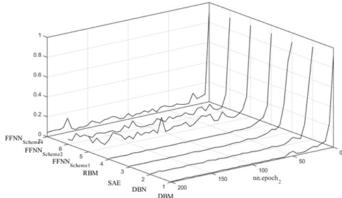
Fig. 9 and Fig. 10 present the convergence process of error rate for data set I and data set II, respectively. For data set I, after only 20 epochs of fine-tuning, the error becomes very small. Fig. 9 shows that the error rate is lower than 0.1 after 50 epochs of fine-tuning for data set II. Compared with the FFNN starting from random initialization (FFNNScheme1~5), Fig. 9 and Fig. 10 also show DNN (DBN, DBM,RBM and SAE) obviously reduce “overfitting” phenomenon for gearbox fault diagnosis. nn.epoch1 and nn.epoch2 are set to 1 and 100 for the following experiment evaluations, respectively.
Fig. 9The error rate on data set I for different classifiers
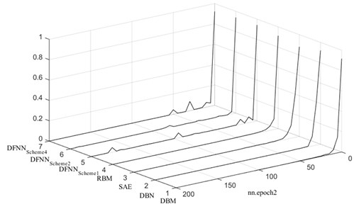
Fig. 10The error rate on data set II for different classifiers
6.2. Performance evaluations
Table 12 presents the classification accuracy by using 8 different classifiers for data set I and II. Compared with FFNN, DBN, DBM, RBM and SAE have better classification performance, especially for data set II.
One or two test cases cannot reflect the reliability and robustness of an algorithm. To further evaluate the performance of DNN, we constructed data set III. Firstly, we consider these data sets (#1-#20), where each one has 12 kinds of different condition patterns (CP = 12, where CP expresses the number of condition patterns included in a data set). Table 13 indicates experiment results by using 8 different classifiers for them. As shown in Table 13, the least classification accuracy among the four DNNs is 92.8 % of SAE for the 15th data set; each of the mean classification accuracy is larger than 98.0 %.
To further challenge the proposed classifiers, we add fault condition pattern included in a data set. Table 14 and 15 present the experiment results of 20 data sets, respectively. Each data set has 20 and 30 kinds of condition patterns respectively (CP = 20 or 30). More condition patterns mean that it is more difficult to obtain good results. As shown in Table 14 and 15, DBN, DBM, RBM and SAE still have good performance for these cases.
Among test cases of 21st-40th data set, DBN, DBM, RBM and SAE have larger than 90 % of mean classification accuracy; the least one is 77.6 % of DBN for the 35th data set. Among test cases of 41st-60th data set, DBN, DBM, RBM and SAE have larger than 84% of mean classification accuracy; the least one is 54.6 % of DBN for the 48th data set.
Table 12Classification accuracy of Data Set I and II
Data set | DBN | DBM | RBM | SAE | FFNNScheme1 | FFNNScheme2 | FFNNScheme4 | SVM |
I | 100 % | 99.94 % | 99.89 % | 99.55 % | 99.66 % | 100 % | 98.33 % | 98.6 % |
II | 98.73 % | 99.06 % | 99.04 % | 99.13 % | 95.46 % | 94.71 % | 96.17 % | 96.5 % |
Table 13Classification accuracy of data set with 12 kinds of condition patterns (CP = 12)
No. | #1 | #2 | #3 | #4 | #5 | #6 | #7 | #8 |
FFNNScheme1 | 63.9 % | 99.0 % | 98.7.0 % | 79.0 % | 98.7 % | 98.7 % | 51.8 % | 98.7 % |
FFNNScheme2 | 61.8 % | 99.4 % | 98.7 % | 62.5 % | 98.8 % | 99.1 % | 55.0 % | 98.0 % |
FFNNScheme4 | 57.3 % | 99.4 % | 99.0 % | 67.0 % | 98.9 % | 99.2 % | 61.8 % | 99.2 % |
SVM | 73.8 % | 96.9 % | 97.8 % | 95.7 % | 98.1 % | 97.4 % | 94.2 % | 97.0 % |
SAE | 97.6 % | 99.2 % | 98.9 % | 99.1 % | 99.0 % | 99.1 % | 99.2 % | 99.4 % |
RBM | 97.3 % | 99.4 % | 98.9 % | 99.2 % | 99.2 % | 99.2 % | 99.3 % | 99.4 % |
DBM | 97.9 % | 99.4 % | 99.0 % | 99.0 % | 99.2 % | 99.2 % | 98.5 % | 99.4 % |
DBN | 95.5 % | 99.4 % | 98.9 % | 99.1 % | 99.3 % | 99.2 % | 99.2 % | 99.5 % |
No. | #9 | #10 | #11 | #12 | #13 | #14 | #15 | #16 |
FFNNScheme1 | 97.4 % | 99.2 % | 98.7 % | 98.7 % | 41.2 % | 98.5 % | 96.8 % | 98.2 % |
FFNNScheme2 | 98.8 % | 99.4 % | 94.5 % | 98.9 % | 41.9 % | 97.3 % | 94.3 % | 99.0 % |
FFNNScheme4 | 96.1 % | 99.4 % | 99.3 % | 99.2 % | 37.1 % | 98.9 % | 96.8 % | 99.0 % |
SVM | 96.3 % | 96.7 % | 97.8 % | 96.5 % | 94.3 % | 97.8 % | 96.8 % | 98.0 % |
SAE | 98.6 % | 99.4 % | 98.8 % | 99.4 % | 92.3 % | 98.6 % | 97.7 % | 99.3 % |
RBM | 98.9 % | 99.2 % | 99.2 % | 99.4 % | 95.5 % | 98.7 % | 98.2 % | 99.4 % |
DBM | 96.4 % | 99.3 % | 98.8 % | 99.5 % | 95.8 % | 99.1 % | 98.1 % | 99.4 % |
DBN | 98.9 % | 99.3 % | 99.4 % | 99.4 % | 94.2 % | 99.1 % | 97.5 % | 99.4 % |
No. | #17 | #18 | #19 | #20 | Mean | Std. | Least | Most |
FFNNScheme1 | 98.4 % | 93.3 % | 92.0 % | 68.0 % | 88.5 % | 17.8 % | 41.3 % | 99.2 % |
FFNNScheme2 | 99.0 % | 93.7 % | 95.2 % | 81.5 % | 88.34 | 17.8 % | 41.9 % | 99.4 % |
FFNNScheme4 | 99.2 % | 93.7 % | 95.0 % | 72.7 % | 88.5 % | 18.4 % | 37.1 % | 99.4 % |
SVM | 95.5 % | 96.3 % | 93.5 % | 96.7 % | 95.3 % | 5.71 % | 71.7 % | 98.1 % |
SAE | 99.2 % | 97.1 % | 94.7 % | 98.9 % | 98.3 % | 1.7 % | 92.8 % | 99.4 % |
RBM | 99.2 % | 95.3 % | 95.1 % | 99.1 % | 98.5 % | 1.4 % | 95.1 % | 99.4 % |
DBM | 99.1 % | 96.8 % | 98.9 % | 98.8 % | 98.3 % | 1.5 % | 93.9 % | 99.5 % |
DBN | 99.1 % | 96.7 % | 96.1 % | 99.3 % | 98.4 % | 1.5 % | 94.2 % | 99.5 % |
6.3. Comparison and analysis
To verify Y. Bengio’s opinion [17, 18] that the gradient-based training of supervised multi-layer neural networks (starting from random initialization) gets easily stuck in “apparent local minima or plateaus”, three multi-layer neural networks (FFNNScheme1, FFNNScheme2, FFNNScheme4) are used to classify the same data set for gearbox fault diagnosis. Their classification results are also indicated in Table 13, 14 and 15, respectively. In addition, SVM is employed to compare with the proposed approaches. The algorithm SVM is applied by using the LibSVM [33]. The parameters for SVM are chosen as 1 and core (kernel) given by a radial basis function where 0.5. These parameters were found through a cross search, aiming at the best model for the SVM.
As shown in Table 13, among 20 test cases CP = 12, three FFNN-based classifiers (FFNNScheme1, FFNNScheme2, and FFNNScheme4) have 5 test cases with bad classification accuracy, even smaller than 70 % for them (#1, #4,#7, #13 and #20), although it is effective for other 14 test cases whose classification accuracies are larger than 90 %. Table 14 indicates that FFNNScheme1, FFNNScheme2, and FFNNScheme4have 4 test cases with bad classification accuracy (#29, #33, #34 and #35). Table 15 indicates that FFNNScheme1, FFNNScheme2, and FFNNScheme4 have 5 test cases (#48, #53, #54, #55 and #57) is bad. This also verifies the negative observations that gradient-based training of multi-layer neural networks (starting from random initialization) gets easily stuck in “apparent local minima or plateaus” in some cases. They don’t have good robustness for gearbox faults diagnosis. Corresponding to the four DNN-based classifiers, they are able to obtain good classification accuracy for 62 data sets. So, we can draw the following conclusions that the DNN-based classifiers are able to avoid falling into “apparent local minima or plateaus” and are reliable and robust for gearbox fault diagnosis. Compared with FFNN-based classifiers and SVM, DBN, DBM,RBM and SAEhave overwhelming superiority in the items of reliability and robustness for gearbox fault diagnosis.
Table 14Classification accuracy of data set with 20 kinds of condition patterns (CP = 20)
No. | #21 | #22 | #23 | #24 | #25 | #26 | #27 | #28 |
FFNNScheme1 | 90.6 % | 93.9 % | 70.0 % | 87.1 % | 90.2 % | 78.2 % | 88.4 % | 77.7 % |
FFNNScheme2 | 93.4 % | 94.0 % | 78.3 % | 91.0 % | 95.2 % | 81.6 % | 96.2 % | 85.1 % |
FFNNScheme4 | 93.2 % | 96.6 % | 80.0 % | 88.4 % | 94.0 % | 84.5 % | 96.4 % | 85.4 % |
SVM | 91.2 % | 90.9 % | 89.0 % | 88.4 % | 92.2 % | 90.3 % | 92.9 % | 85.6 % |
SAE | 95.7 % | 95.8 % | 90.3 % | 93.3 % | 96.3 % | 83.2 % | 96.6 % | 86.9 % |
RBM | 95.3 % | 96.3 % | 92.3 % | 94.5 % | 96.6 % | 85.4 % | 97.1 % | 88.7 % |
DBM | 95.5 % | 96.4 % | 92.7 % | 93.9 % | 96.2 % | 85.7 % | 96.9 % | 88.4 % |
DBN | 94.2 % | 96.8 % | 90.4 % | 93.8 % | 96.4 % | 85.1 % | 96.6 % | 87.4 % |
No. | #29 | #30 | #31 | #32 | #33 | #34 | #35 | #36 |
FFNNScheme1 | 67.2 % | 86.9 % | 87.9 % | 73.3 % | 57.2 % | 59.2 % | 45.9 % | 75.7 % |
FFNNScheme2 | 70.7 % | 86.0 % | 94.8 % | 91.0 % | 57.6 % | 76.6 % | 52.1 % | 83.4 % |
FFNNScheme4 | 78.0 % | 88.8 % | 96.3 % | 82.3 % | 64.9 % | 74.4 % | 62.1 % | 82.9 % |
SVM | 76.8 % | 88.2 % | 91.6 % | 88.1 % | 78.3 % | 90.4 % | 59.4 % | 79.5 % |
SAE | 84.8 % | 91.5 % | 97.2 % | 93.3 % | 83.9 % | 90.1 % | 80.4 % | 84.5 % |
RBM | 84.6 % | 91.8 % | 97.0 % | 93.8 % | 91.7 % | 89.5 % | 80.2 % | 85.6 % |
DBM | 86.9 % | 91.9 % | 97.1 % | 93.2 % | 89.7 % | 89.4 % | 81.7 % | 84.2 % |
DBN | 86.4 % | 92.3 % | 96.7 % | 93.1 % | 81.7 % | 88.1 % | 77.6 % | 85.2 % |
No. | #37 | #38 | #39 | #40 | Mean | Std. | Least | Most |
FFNNScheme1 | 71.2 % | 87.4 % | 80.6 % | 85.2 % | 77.7 % | 12.9 % | 45.9 % | 93.9 % |
FFNNScheme2 | 79.6 % | 89.7 % | 88.9 % | 89.4 % | 83.7 % | 12.0 % | 52.1 % | 96.2 % |
FFNNScheme4 | 84.4 % | 93.7 % | 84.2 % | 94.0 % | 85.2 % | 9.9 % | 62.1 % | 96.6 % |
SVM | 84.6 % | 90.3 % | 85.9 % | 92.9 % | 86.3 % | 7.92 % | 59.4 % | 92.9 % |
SAE | 87.8 % | 95.5 % | 91.6 % | 95.0 % | 90.7 % | 5.2 % | 80.4 % % | 97.2 % |
RBM | 90.4 % | 95.8 % | 91.4 % | 96.0 % | 91.7 % | 4.8 % | 80.2 % | 97.1 % |
DBM | 90.9 % | 95.9 % | 91.1 % | 96.4 % | 91.7 % | 4.6 % | 81.7 % | 97.1 % |
DBN | 90.7 % | 95.7 % | 91.3 % | 94.9 % | 90.7 % | 5.4 % | 77.6 % | 96.8 % |
As for the comparison between SAE, RBM, DBM and DBN, Fig.11 indicates the mean classification accuracy data set with different kinds of condition patterns (CP = 12, 20 and 30) for SAE, RBM, DBM and DBN, respectively. As shown in Fig. 11, four deep neural networks have almost equal classification accuracy for the data set with CP = 12; in the case of CP = 20 and 30, RBM and DBM are slightly better than SAE and DBN. However, the classification accuracy of SAE, RBM, DBM and DBN need to be further enhanced for the data set that includes condition patterns more than 20 kinds.
Fig. 11Comparison between SAE, RBM, DBM and DBN
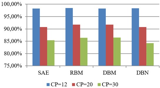
Table 15Classification accuracy of data set with 30 kinds of condition patterns (CP = 30)
No. | #41 | #42 | #43 | #44 | #45 | #46 | #47 | #48 |
FFNNScheme1 | 84.1 % | 79.9 % | 65.7 % | 72.8 % | 63.6 % | 70.9 % | 86.3 % | 68.3 % |
FFNNScheme2 | 85.6 % | 88.7 % | 85.7 % | 69.6 % | 83.2 % | 82.3 % | 65.1 % | 33.9 % |
FFNNScheme4 | 75.9 % | 87.3 % | 87.8 % | 66.6 % | 73.9 % | 88.3 % | 77.0 % | 36.0 % |
SVM | 87.9 % | 85.2 % | 84.2 % | 56.5 % | 86.9 % | 85.0 % | 80.6 % | 62.0 % |
SAE | 86.6 % | 89.2 % | 87.7 % | 82.5 % | 85.0 % | 92.6 % | 85.8 % | 69.0 % |
RBM | 89.6 % | 91.6 % | 86.8 % | 82.2 % | 86.6 % | 93.3 % | 87.5 % | 70.8 % |
DBM | 88.5 % | 91.4 % | 87.8 % | 81.9 % | 86.8 % | 92.8 % | 89.0 % | 69.5 % |
DBN | 90.8 % | 92.3 % | 86.5 % | 77.4 % | 86.8 % | 92.6 % | 84.7 % | 54.6 % |
No. | #49 | #50 | #51 | #52 | #53 | #54 | #55 | #56 |
FFNNScheme1 | 51.0 % | 78.5 % | 85.0 % | 61.2 % | 38.8 % | 48.6 % | 30.4 % | 54.4 % |
FFNNScheme2 | 80.9 % | 41.6 % | 88.7 % | 70.0 % | 83.4 % | 86.0 % | 74.3 % | 85.5 % |
FFNNScheme4 | 76.8 % | 53.4 % | 87.2 % | 71.8 % | 83.2 % | 87.4 % | 68.6 % | 88.3 % |
SVM | 84.2 % | 56.6 % | 90.0 % | 80.9 % | 82.0 % | 86.6 % | 73.4 % | 89.5 % |
SAE | 88.6 % | 73.0 % | 90.8 % | 85.0 % | 89.6 % | 88.5 % | 83.6 % | 90.4 % |
RBM | 90.0 % | 71.6 % | 92.8 % | 84.9 % | 90.2 % | 91.2 % | 83.4 % | 91.3 % |
DBM | 89.6 % | 76.9 % | 92.4 % | 86.1 % | 91.3 % | 90.0 % | 83.5 % | 90.8 % |
DBN | 88.9 % | 65.4 % | 90.9 % | 86.5 % | 90.9 % | 90.8 % | 79.4 % | 90.0 % |
No. | #57 | #58 | #59 | #60 | Mean | Std. | Least | Most |
FFNNScheme1 | 57.3 % | 82.1 % | 65.4 % | 76.2 % | 66.0 % | 15.7 % | 30.4 % | 86.3 % |
FFNNScheme2 | 39.4 % | 64.2 % | 55.7 % | 71.7 % | 71.8 % | 17.1 % | 33.8 % | 88.7 % |
FFNNScheme4 | 86.4 % | 77.4 % | 64.2 % | 78.5 % | 75.8 % | 13.4 % | 36.0 % | 88.3 % |
SVM | 85.2 % | 88.3 % | 67.1 % | 83.9 % | 79.8 % | 10.7 % | 55.5 % | 90.0 % |
SAE | 92.6 % | 84.5 % | 73.3 % | 89.0 % | 85.4 % | 6.5 % | 69.0 % | 92.6 % |
RBM | 93.7 % | 86.6 % | 73.1 % | 90.1 % | 86.4 % | 7.0 % | 70.8 % | 93.7 % |
DBM | 93.3 % | 86.4 % | 70.5 % | 91.3 % | 86.5 % | 6.9 % | 69.5 % | 93.3 % |
DBN | 93.0 % | 87.5 % | 68.4 % | 87.4 % | 84.2 % | 10.3 % | 54.6 % | 93.0 % |
7. Conclusions
In this paper, based on 62 data sets corresponding to the various health conditions of two rotating mechanical systems, four deep learning algorithms including RBM, DBM, DBN and SAE are extensively evaluated for vibration-based gearbox fault diagnosis. Some interesting findings from this study are given below:
1) Multi-layer feed-forward neural network with one or two hidden layers performs better than deeper net architectures for gearbox fault diagnosis, and they are prone to be stuck in “apparent local minima or plateaus” in the test cases. As a result, they don’t show good robustness for gearbox faults diagnosis.
2) The testing results demonstrate that the deep learning algorithms, RBM, DBM, DBN and SAE, are efficient, reliable and robust in gearbox fault diagnosis. These classifiers have a good potential to provide helpful maintenance guidelines for industrial systems. With these methods, different types of component faults at different severity levels (e.g., initial stage or advanced stage) could be well classified. Furthermore, it is also shown that vibration signals usually carry rich information in fault detection, control and maintenance planning of rotating machines.
References
-
Cerrada M., Sánchez R. V., Cabrera D., Zurita G., Li C. Multi-stage feature selection by using genetic algorithms for fault diagnosis in gearboxes based on vibration signal. Sensor, Vol. 15, 2015, p. 23903-23926.
-
Lei Y., Zuo M. J., He Z., Zi Y. A multidimensional hybrid intelligent method for gear fault diagnosis. Expert Systems with Applications, Vol. 37, 2010, p. 1419-1430.
-
Li Chuan, Cabrera Diego, de Oliveira José Valente, Sanchez René Vinicio, Cerrada Mariela, Zurita Grover Extracting repetitive transients for rotating machinery diagnosis using multiscale clustered grey infogram. Mechanical Systems and Signal Processing, Vol. 76-77, 2016, p. 157-173.
-
Wang D., Miao Q., Kang R. Robust health evaluation of gearbox subject to tooth failure with wavelet decomposition. Journal of Sound and Vibration, Vol. 324, Issues 3-5, 2009, p. 1141-1157.
-
Yuan J., He Z., Zi Y., Liu H. Gearbox fault diagnosis of rolling mills using multiwavelet sliding window neighboring coefficient denoising and optimal blind deconvolution. Science in China Series E: Technological Sciences, Vol. 52, 2009, p. 2801-2809.
-
Yu Fajun, Zhou Fengxing Classification of machinery vibration signals based on group sparse representation. Journal of Vibroengineering, Vol. 18, Issue 3, 2016, p. 1459-1473.
-
Li C., Liang M. Time-frequency signal analysis for gearbox fault diagnosis using a generalized synchrosqueezing transform. Mechanical Systems and Signal Processing, Vol. 26, 2012, p. 205-217.
-
Guo L., Chen J., Li X. Rolling bearing fault classification based on envelope spectrum and support vector machine. Journal of Vibration and Control, Vol. 15, Issue 9, 2009, p. 1349-1363.
-
Chen F., Tang B., Chen R. A novel fault diagnosis model for gearbox based on wavelet support vector machine with immune genetic algorithm. Measurement, Vol. 46, Issue 1, 2013, p. 220-232.
-
Yang Z., Hoi W. I., Zhong J. Gearbox fault diagnosis based on artificial neural network and genetic algorithms. International Conference on System Science and Engineering, 2011, p. 37-42.
-
Tayarani-Bathaie S. S., Vanini Z. N. S., Khorasani K. Dynamic neural network-based fault diagnosis of gas turbine engines. Neurocomputing, Vol. 125, Issue 11, 2014, p. 153-165.
-
Ali J. B., Fnaiech N., Saidi L., Chebel-Morello B., Fnaiech F. Application of empirical mode decomposition and artificial neural network for automatic bearing fault diagnosis based on vibration signals. Applied Acoustics, Vol. 89, 2015, p. 16-27.
-
Abu-Mahfouz I. A comparative study of three artificial neural networks for the detection and classification of gear faults. International Journal of General Systems, Vol. 34, Issue 3, 2009, p. 261-277.
-
Souza1 D. L., Granzotto M. H., Almeida G. M., Oliveira-Lopes L. C. Fault detection and diagnosis using support vector machines – a SVC and SVR comparison. Journal of Safety Engineering, Vol. 3, Issue 1, 2014, p. 18-29.
-
Bengio Y., Lamblin P., Popovici D., Larochelle H. Greedy layer-wise training of deep networks. Advances in Neural Information Processing Systems 19, MIT Press, 2007, p. 153-160.
-
Erhan D., Manzagol P.-A., Bengio Y., Bengio S., Vincent P. The difficulty of training deep architectures and the effect of unsupervised pretraining. Proceedings of 12th International Conference on Artificial Intelligence and Statistics, 2009, p. 153-160.
-
Jia Feng, Lei Yaguo, Lin Jing, Zhou Xin, Lu Na Deep neural networks: a promising tool for fault characteristic mining and intelligent diagnosis of rotating machinery with massive data. Mechanical Systems and Signal Processing, Vol. 72-73, 2016, p. 303-315.
-
Freund Y., Haussler D. Unsupervised Learning of Distributions on Binary Vectors Using Two Layer Networks. Technical Report UCSC-CRL-94-25, University of California, Santa Cruz, 1994.
-
Hinton G. E., Osindero S., Teh Y. A fast learning algorithm for deep belief nets. Neural Computation, Vol. 18, 2006, p. 1527-1554.
-
Bengio Y. Learning deep architectures for AI. Foundations and Trends in Machine Learning, Vol. 2, Issue 1, 2009, p. 1-127.
-
Tran V. T., Thobiani F. A., Ball A. An approach to fault diagnosis of reciprocating compressor valves using Teager-Kaiser energy operator and deep belief networks. Expert Systems with Applications, Vol. 41, 2014, p. 4113-4122.
-
Tamilselvan P., Wang P. Failure diagnosis using deep belief learning based health state classification. Reliability Engineering and System Safety, Vol. 115, 2013, p. 124-135.
-
Li C., Sanchez R., Zurita G., Cerrada M., Cabrera D., Vásquez R. Multimodal deep support vector classification with homologous features and its application to gearbox fault diagnosis. Neurocomputing, Vol. 168, 2015, p. 119-127.
-
Chen Z., Li C., Sánchez R. V. Multi-layer neural network with deep belief network for gearbox fault diagnosis. Journal of Vibroengineering, Vol. 17, Issue 5, 2015, p. 2379-2392.
-
Li Chuan, Liang Ming, Wang Tianyang Criterion fusion for spectral segmentation and its application to optimal demodulation of bearing vibration signals. Mechanical Systems and Signal Processing, Vol. 64, Issue 65, 2015, p. 132-148.
-
Deng Li, Hinton Geoffrey, Kingsbury Brian New types of deep neural network learning for speech recognition and related applications: an overview. IEEE International Conference on Acoustics, Speech, and Signal Processing (ICASSP), May 2013.
-
Vincent P., Larochelle H., Lajoie I., Bengio Y., Manzagol P. A. Stacked denoising autoencoders: learning useful representations in a deep network with a local denoising criterion. Journal of Machine Learning Research, Vol. 11, 2010, p. 3371-3408.
-
Salakhutdinov R. R., Hinton G. E. Deep Boltzmann machines. Proceedings of the International Conference on Artificial Intelligence and Statistics, 2009.
-
Hinton G. E. Training products of experts by minimizing contrastive divergence. Neural Computation, Vol. 14, Issue 8, 2002, p. 1771-1800.
-
Cho K. H., Ilin A., Raiko T. Improved learning of Gaussian-Bernoulli restricted Boltzmann machines. Lecture Notes in Computer Science, Vol. 6791, 2011, p. 10-17.
-
Bourlard H., Kamp Y. Auto-association by multilayer perceptrons and singular value decomposition. Biological Cybernetics, Vol. 59, 1988, p. 291-294.
-
Vincent P., Larochelle H., Bengio Y., Manzagol P.-A. Extracting and composing robust features with denoising autoencoders. Proceedings of the 25th International Conference on Machine Learning, ACM, 2008, p. 1096-1103.
-
Chang C. C., Lin C. J. LIBSVM: a library for support vector machines. ACM Transactions on Intelligent Systems and Technology, 2013.
Cited by
About this article

This work is supported by Scientific and Technological Research Program of Chongqing Municipal Education Commission (No. KJ1500607), Science Research Fund of Chongqing Technology and Business University (No. 2011-56-05(1153005)), Science Research Fund of Chongqing Engineering Laboratory for Detection Control and Integrated System (DCIS20150303), the National Natural Science Foundation of China (51375517, 61402063), the Project of Chongqing Innovation Team in University (KJTD201313) and Natural Science Foundation Project of CQ CSTC (No. cstc2013kjrc-qnrc40013).
Xudong Chen coded for DBM algorithm; Chuan Li coded for SAE algorithm; René-Vinicio Sanchez collected the vibration signals from the gearbox fault digressions experiment platform; Huafeng Qin extracted the features of the vibration signals.
