Improved genetic algorithm for parameters identification of cart-double pendulum

Dan, Yuanhong; Xu, Peng; Zhang, Wei; Tan, Zhi

doi:10.21595/jve.2019.20663

Journal of Vibroengineering

Browse Journal

Submit article

Published: 30 September 2019

Check for updates

Improved genetic algorithm for parameters identification of cart-double pendulum

Yuanhong Dan¹

Peng Xu²

Wei Zhang³

Zhi Tan⁴

^{1, 2, 3, 4}Chongqing University of Technology, Chongqing, China

Corresponding Author:

Peng Xu

Cite the article Download PDF

Downloads 1439

WoS Core Citations 3

CrossRef Citations 3

Abstract

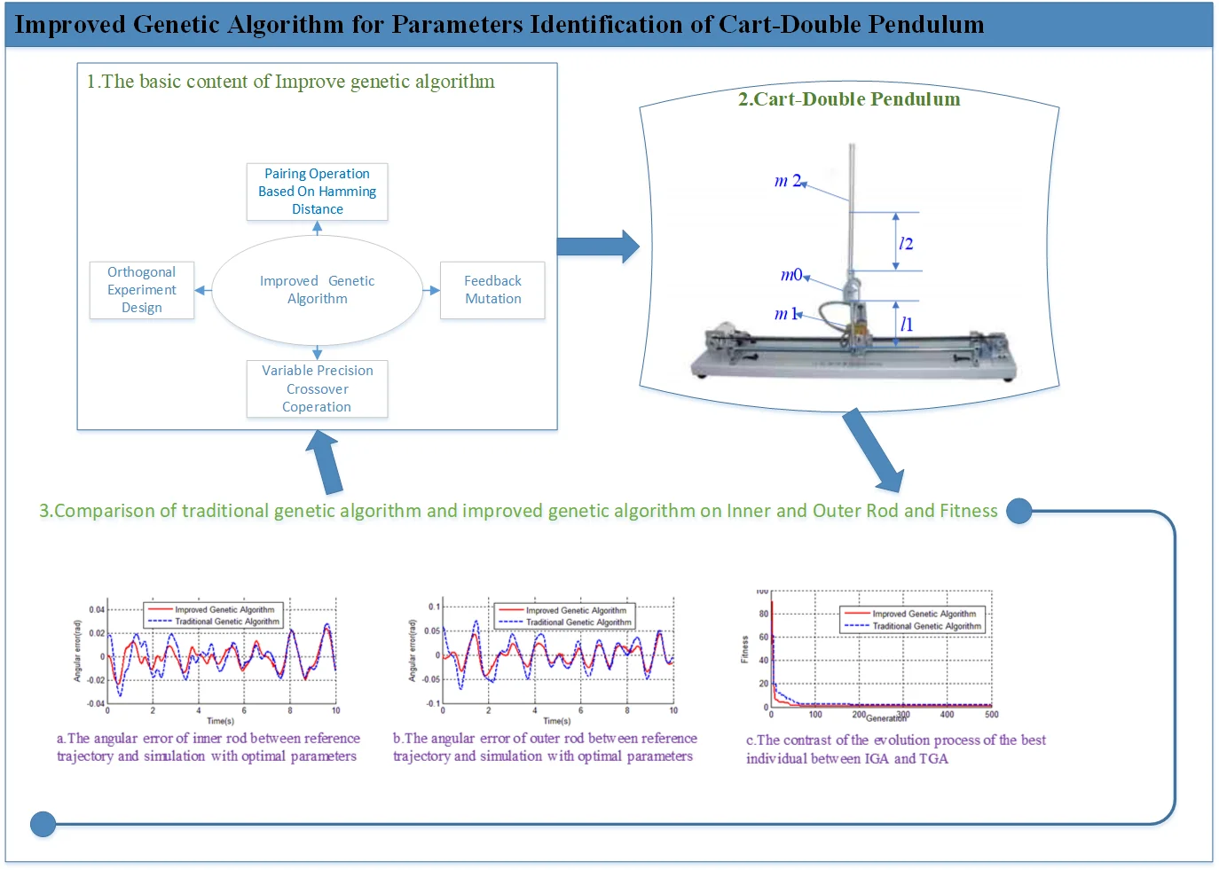
Cart-double pendulum is a typical nonlinear under-actuated mechanical device, and highly sensitive to modeling error and external disturbance. Motion control of double pendulum is a very complex and difficult task, especially when it turns to real-time situation because a minor difference between kinetic model and actual device could lead to the necessity of significant adjustments according to control laws comparing to the usage of simulation controller. The use of accurate kinetic model is the key factor for fast transition from simulation to real-time operation. An improved genetic algorithm (IGA), which includes orthogonal experiment design, feedback mutation, pairing operation based on Hamming distance, and variable precision crossover operation, is introduced to identify the physical parameters of a double pendulum. The improved genetic algorithm (IGA) can overcome the shortcomings of the traditional genetic algorithm (TGA), for instance, premature convergence, and get results closer to the global optimal solution. The results of experiments demonstrate the effectiveness of the proposed method.

Improved genetic algorithm for parameters identification of cart-double pendulum

1. Introduction

Multi-inverted pendulum is a typically nonlinear, multi-variable, strongly coupled, under-actuated mechanical system, which has been recognized as a classical platform for validating a new control method and control algorithm. Because of the properties of simple structure, low cost, and high control difficulty, multi-inverted pendulum related research has always been one of the hotspots in the control field. The researches of multi-inverted pendulum can be classified into 3 categories: (a) balance control in the neighborhood of inverted equilibrium point; (b) swing-up control from downward equilibrium to inverted equilibrium; (c) arbitrary transfer control from one equilibrium state to another. Balance control has been achieved from single pendulum to four-inverted pendulum [1-3], however, most researches on swing-up control and arbitrary transfer control still focus on the simulation [4-7], and few real-time researches are reported [8-10]. One obstacle is under-actuation characteristic, because rods can be controlled only indirectly through the movement of cart, that makes inverted pendulum be very sensitive to disturbance, and the controllability is very low. Another challenge is that a simulation result cannot be directly applied to the real-time control, because the mathematic model is not equivalent to the device. Owing to the sensibility and low-controllability of rods, a minor difference of controlled object between simulation and real-time control can lead to the necessity to make major adjustments of control parameters, even to redesign the controller configuration.

So, the accurate kinetic model is the key to speed up the process of transition from simulation control to real-time control. Traditional method to build up a kinetic model is to set up the model structure by applying a physics law (such as energy conservation law and momentum conservation law), and then get the values of physical parameters by direct measurement. It is difficult to obtain an accurate model with the help of the traditional method, because of the following reasons:

(1) Some idealized assumptions lead to a structural model error. Such as, all components of mechanical system are treated as a homogeneous rigid body, small volume parts are simplified as particles. There also could be unmodeled dynamics, as the manufacturing, assembling, and operating environments of a mechanical system always include unknown factors.

(2) Some physical parameters (such as mess, length, etc.) can be measured directly, while some parameters (such as moment of inertia, centroid position, friction coefficient, etc.) are difficult to be measured directly. Because of unmodeled dynamics, even for the parameters that can be measured directly, the appropriate adjustments shall be made to narrow down the difference caused by the unmodeled dynamics.

It is impractical to try to figure out all the unmodeled dynamics and to find out the real values of each parameter manually. This paper introduced a more effective and realistic modeling method which combined the idea of quasi-equivalent modeling [11] with the improved genetic algorithm. The main ideas of the proposed method include:

(1) If a mathematic model can reflect the main characteristics of actual device, then we can say the simulation environment is equivalent to the real-time environment, which means the controller effective in simulation will be also effective in the real time.

(2) The main characteristics are always contained in typical response data, such as step response, zero input response, etc. The difference between two systems can be quantized by the typical response data of those two systems. The smaller the difference is, the closer those two systems approach to the appropriate result.

(3) The improved genetic algorithm is used to search equivalent physical parameters for a kinetic model. Fitness function is established with the idea the same as in (2), feedback mutation is used to enhance the diversity of population, so the orthogonal experiment is applied to increase the searching efficiency; the variable-precision crossover is introduced to improve the searching accuracy, and the hamming distance is introduced to avoid inbreeding.

Genetic algorithm (GA) is a heuristic scientific method based on the Darwin’s biological evolution theory [12], which has been widely applied to solve the high dimensional optimization problem for parameter optimization in engineering and science areas. However, because of the contradiction between the high dimension of the population and the limited settlement space, the traditional genetic algorithm has the problems of inbreeding and premature convergence, and easily falls into local optimal solution [13]. The proposed improved genetic algorithm in (3) can greatly overcome these defects. The experimental results of manual trial, traditional genetic algorithm, and improved genetic algorithm are provided to validate the effectiveness of the proposed method.

The rest of this paper is organized as follows: Section 2 describes the structure and mathematic model of CDP; In Section 3, the methods are proposed for the improvement to traditional GA; Section 4 shows the experimental results and the discussion; Section 5 addresses the conclusions of the note.

2. Physical structure and mathematic model of cart double pendulum

A typical cart double pendulum device is shown in Fig. 1; its physical structure is shown in Fig. 2. The degree of freedom of Cart-Double Inverted Pendulum is 3 (cart, inner rod, and outer rod), while only one servo motor is applied to drive the cart move back and forth within a limited straight track. The joint between cart and inner rod, and the joint between inner rod and outer rod, are passive links which can only be under the influence of the coupling effect of the joints. The angles of joints are detected by encoders which are on each link.

The cart displacement is $x$ , the angle of inner rod is $θ_{1}$ , the angle of outer rod is $θ_{2}$ . The generalized variables are taken as $q = [\begin{array}{l} x & θ_{1} & θ_{2} \end{array}]^{T}$ , then $\dot{q} = [\begin{array}{l} \dot{x} & {\dot{θ}}_{1} & {\dot{θ}}_{2} \end{array}]^{T}$ . The kinetic model of cart double pendulum can be derived by dynamic analysis method as follows [14]:

1

[\begin{array}{l} 1 & 0 & 0 \\ A_{21} & A_{22} & A_{23} \\ A_{31} & A_{32} & A_{33} \end{array}] \ddot{q} + [\begin{array}{l} 0 & 0 & 0 \\ 0 & C_{22} & C_{23} \\ 0 & C_{32} & C_{33} \end{array}] \dot{q} = [\begin{matrix} u \\ (m_{1} l_{1} + m_{2} L + m_{0} L) g s i n θ_{1} \\ m_{2} g l_{2} s i n θ_{2} \end{matrix}],

where:

A_{21} = (m_{1} l_{1} + m_{2} L + m_{0} L) c o s θ_{1}, A_{22} = m_{1} l_{1}^{2} + J_{1} + m_{2} L^{2} + m_{0} L^{2}

A_{23} = A_{32} = m_{2} L l_{2} c o s (θ_{1} - θ_{2}), A_{31} = m_{2} l_{2} c o s θ_{2}, A_{33} = m_{2} l_{2}^{2} + J_{2},

C_{22} = c_{1} + c_{2}, C_{23} = m_{2} L l_{2} {\dot{θ}}_{2} s i n (θ_{1} - θ_{2}) - c_{2},

C_{32} = - m_{2} L l_{2} {\dot{θ}}_{2} s i n (θ_{1} - θ_{2}) - c_{2}, C_{33} = c_{2} .

Fig. 1Experimental facilities of cart double pendulum

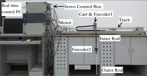
Fig. 2Physical structure of cart double pendulum

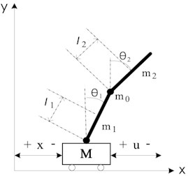
Physical meaning of each variable is shown in Table 1.

Among these physical parameters in Table 1, the length ( $L$ ) and mass ( $m_{1}$ , $m_{2}$ , $m_{0}$ ) can be easily measured directly; while the centroid position ( $l_{1}$ , $l_{2}$ ) and moment of inertia ( $J_{1}$ , $J_{2}$ ) are not so easy to be measured. If we take the rod as a homogeneous rigid body, the centroid position and moment of inertia can be calculated according to the mass and length of each rod. The rotational friction coefficients ( $c_{1}$ , $c_{2}$ ) are very hard to be measured, and they can only be estimated according to experience or factory parameters of the bearing. The estimated values for physical parameters of cart double pendulum are shown in Table 2.

Table 1Physical parameters of cart double pendulum

Parameter	Physical meaning
$m_{1}$ , $m_{2}$ , $m_{0}$	Mass of inner rod, outer rod, and encoder
$L$	Length of inner rod and outer rod
$J_{1}$ , $J_{2}$	Moment of inertia of inner rod, and outer rod
$l_{1}$ , $l_{2}$	Centroid position of inner rod, and outer rod
$c_{1}$	Rotational friction of cart-inner rod axis
$c_{2}$	Rotational friction of inner rod-outer rod axis
$u$	Control variable

Table 2Estimated values for physical parameters of cart double pendulum

Parameter	Value	Parameter	Value
$L$ (m)	0.4	$m_{2}$ (kg)	0.108
$l_{1}$ (m)	0.2	$m_{0}$ (kg)	0.208
$l_{2}$ (m)	0.2	$c_{1}$	0.00705
$m_{1}$ (kg)	0.108	$c_{2}$	0.00305
$J_{2}$ (kg.m²)	0.00133	$J_{1}$ (kg.m²)	0.00133

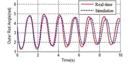
It is required to confirm how much the estimated values in Table 2 can represent the actual device. Like the idea shown in Section 1, both simulation model and actual device in the same initial state (shown in Table 3) are made, and the zero input response data of simulation and real-time are recorded. The contrast cures are shown in Fig. 3 and Fig. 4.

Table 3Initial state of cart double pendulum

State variable	Value	State variable	Value
$x$	0.000	$\dot{x}$	0.000
$θ_{1}$	3.36093	${\dot{θ}}_{1}$	–3.45705
$θ_{2}$	3.88832	${\dot{θ}}_{2}$	11.15684

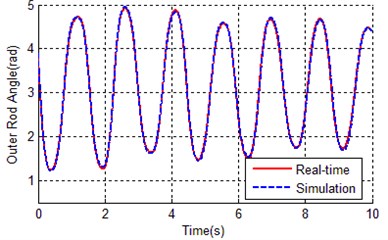
Fig. 3 and Fig. 4 respectively show the contrast curves of inner rod and outer rod. As it can be seen from Fig. 3 and Fig. 4, the basic trend of zero input response between simulation and real time is the same, but also there are obvious differences in swing period and vibrating amplitude. This means the values in Table 2 have certain representativeness, but not the accuracy enough to equivalent to actual device. In order to make simulation environment equivalent to the real time environment, we need to find out more accurate parameters for kinetic model (Eq. (1)).

Fig. 3Contrast of inner rod angle between real time and simulation

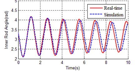
Fig. 4Contrast of outer rod angle between real time and simulation

3. Improved genetic algorithm

As mentioned in Section 1, the genetic algorithm is introduced to search for the optimal physical parameter values, and some improvements are put forward to overcome the defects of the traditional genetic algorithm (such as inbreeding and premature convergence). Details are shown bellow.

3.1. Pairing operation based on Hamming distance

Hamming distance is introduced to calculate the difference between two individuals (chromosomes). Considering that two chromosomes are $x = \{x_{1}, x_{2}, \dots, x_{N}\}$ and $y = {y_{1}, y_{2}, \dots, y_{N}}$ , the hamming distance of $x$ and $y$ can be calculated as follows:

2

D_{H a i m i n g} (x, y) = \sum_{i = 1}^{N} d_{i},

where, $d = {d_{1}, d_{2}, \dots, d_{N}}$ , $d_{i} = \{\begin{matrix} \begin{matrix} 1, & x_{i} \neq y_{i}, \end{matrix} \\ \begin{matrix} 0, & x_{i} = y_{i} \end{matrix} . \end{matrix}$

If $D_{H a i m i n g} (x, y) \leq 1$ , then $x$ and $y$ are forbidden to pairing and crossover to produce offspring, and chromosome $y$ is regenerated by the following method:

3

y_{i} = L_{i} + β (U_{i} - L_{i}),

where $L_{i}$ and $U_{i}$ are respectively the lower limited value and upper limited value of the $i$ th gene (parameter), $β \in {0.0,0.1,0.2, \dots, 0.9,1.0}$ . The introduction of hamming distance can increase the diversity of population and avoid inbreeding.

3.2. Variable precision crossover

The traditional crossover operation only involves genetic exchange of parental chromosomes according to the crossover point; this is an obstacle for searching precision. Considering two chromosomes $x$ and $y$ , the offsprings of $x$ and $y$ are generated with variable precision crossover operation as follows:

4

x^{'} = \{x_{1}, x_{2}, \dots, x_{i}^{'}, y_{i + 1}, \dots, y_{N}\}, y^{'} = \{y_{1}, y_{2}, \dots, y_{i}^{'}, x_{i + 1}, \dots, x_{N}\},

where: $x_{i}^{'} = x_{i} + β (y_{i} - x_{i})$ , $y_{i}^{'} = L_{i} + β (U_{i} - L_{i})$ , $i$ is the index of crossover point, $β$ is a random number and $β \in {0.0,0.1,0.2, \dots, 0.9,1.0}$ . This method of dynamically expanding precision allows searching for a feasible solution from a low-precision solution space to a high-precision solution space, to further enhance chromosome diversity.

3.3. Orthogonal experiments in crossover operation

Orthogonal experiments are adopted to speed up the evolutionary process of genetic algorithm. Orthogonal experiment is a kind of efficient and economical experimental method which deals with multiple factors and multiple levels by means of orthogonal table. The best offspring of two ancestor chromosomes can be obtained through lesser experiments if the orthogonal experiment method is adopted [15].

Here, two-level orthogonal experiments are used. When the orthogonal table is selected, if the column number of orthogonal table is greater than the number of variable, then the spare columns are just abscised. Each factor has two levels (the number of value fetch choice), which respectively correspond to the two values of the corresponding gene in a chromosome. A new table with the same dimension of selected orthogonal table is filled with another value according to the value in the orthogonal table and the value range of relevant gene, and the number of experiments is equal to the row number of orthogonal table. The optimal combination of multiple variables can be obtained by means of experiment arrangement method of orthogonal table.

Two chromosomes are selected randomly to perform the orthogonal experiment after the crossover operation, so as to find out the optimal level (parameter value) for each factor, and the optimal chromosome can be formed with these optimal levels for each factor. Then, the best offspring of ancestor chromosomes is produced.

3.4. Feedback mutation

As the evolutionary process continues, more and more offsprings are generated by good individuals, and the individuals in population tend to be the same, so this leads to the lack of genetic diversity. Then the evolutionary process becomes very slow, even stops, especially at the later stage of evolution, population falls into premature convergence. By replacing highly similar individuals with randomly generated new individuals, the diversity of population will increase, but the evolutionary process will also become a random process and will have no possibility of convergence to global optimal solution.

Feedback mutation is performed according to the population fitness: if the population fitness is bigger than a given consistent $α$ , then feedback mutation is activated; otherwise feedback mutation is disabled. Population fitness is calculated as follows:

5

f_{p o p u l a t i o n} = \frac{\sum_{i = 1}^{M} f_{i}}{M \times f_{o p t i m a l}},

where, $f_{o p t i m a l}$ is the fitness of the best individual; $M$ is the size of population; $f_{i}$ is the fitness of the $i$ th chromosome in population.

The new individual is generated by the following method:

6

y_{i} = μ ∙ x_{i} + β ∙ ν ∙ x_{i},

where, $y_{i}$ is the $i$ th gene of new generated individual; $μ$ and $ν$ are given consistent less than 1; $x_{i}$ is the $i$ th gene of the best individual in population; $β$ is a random number, and $β \in {0,0.1, \dots, 1}$ .

Feedback mutation is intended to overcome fundamentally the premature convergence of the population. In the later stage of population optimization, the replacement of the individuals that have been eliminated by mutation with new randomly generated individuals can greatly improve the population diversity while maintaining the stability of the population size.

3.5. Nonlinear transformation of fitness function

Fitness function is used to evaluate the quality of an individual in the genetic algorithm; the fitness value directly determines the reproductive opportunities of a certain individual. So, the fitness function is very important for the genetic algorithm and needs targeted design according to a specific question. Considering two situations, individuals with low fitness may be eliminated before they have a chance to perform the genetic operation; while the offspring generated by individuals with high fitness will fill up the whole population. This is bad for population diversity, and the fitness function shall be transformed to give a certain survival chance to a low fitness individual. The solution is to reduce the difference between the chromosomal fitness values by a logarithmic function. The nonlinear transformation of the fitness function is as follows:

7

H (x) = \{\begin{array}{l} δ - 10 l o g C, & f (x) > C, \\ δ - 10 l o g f (x), & f (x) \leq C, \end{array}

where, $H (x)$ is the new fitness function, $f (x)$ is the original fitness function, $δ$ and $C$ are consistent to make sure that $H (x)$ is positive, and to regulate the possibility of poor chromosomes and better chromosomes being selected for the crossover or mutation operation.

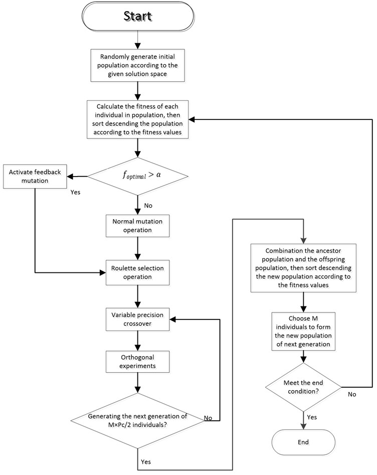
3.6. Process of improved genetic algorithm

Step 1: randomly generate initial population according to the given solution space.

Step 2: calculate the fitness of each individual in population, then sort descending the population according to the fitness values.

Step 3: calculate the fitness of population. If $f_{o p t i m a l} > α$ , then activate feedback mutation, otherwise only the normal mutation operation is used.

Step 4: roulette selection operation.

Step 5: variable precision crossover.

Step 6: orthogonal experiments.

Step 7: repeat steps 5-7 until $M$ × $P c$ /2 individuals of the next generation are generated.

Step 8: combine the ancestor population and the offspring population, then sort descending the new population according to the fitness values.

Step 9: choose $M$ individuals to form a new population of next generation.

Step 10: finish if the terminal conditions are met, otherwise repeat steps 3-10.

Fig. 5 contains a flow chart of the improved genetic algorithm.

Fig. 5Flow chart of improved genetic algorithm

4. Experimental results

In this section, the kinetic parameters identification of cart double pendulum will be performed with both the traditional genetic algorithm (TGA) and the improved genetic algorithm (IGA). For the comparative purpose, we use the same gene coding method (real coding) and fitness function for both TGA and IGA.

4.1. Chromosome and fitness function

The physical parameters of cart double pendulum are shown in Table 1, and the estimated values are shown in Table 2. The length of rods ( $L$ ) is assured, and shall not be optimized; mass parameters ( $m_{1}$ , $m_{2}$ , $m_{0}$ ) can be measured directly, but shall be adjusted to compromise the unmodeled dynamics; the other parameters ( $c_{1}$ , $c_{2}$ , $l_{1}$ , $l_{2}$ , $J_{1}$ , $J_{2}$ ) cannot measured directly. So, the genes in chromosome can be selected as follows:

8

Z = (m_{1}, m_{1}, m_{0}, l_{1}, l_{2}, J_{1}, J_{2}, c_{1}, c_{2}),

where $Z$ is a chromosome in the genetic algorithm, which contains the physical parameters to be identified, each parameter is coded with double-precison real number. $Z \subset [L, U]$ defines the solution space of parameters, $L$ is lower limit, and $U$ is upper limit. The estimated value in Table 2 are not accuracy enough to represent the actual device, but the basic trend is in the line with actual situation, so the solution space can be expanded based on the values from Table 2:

9

L = (0.216, 0.216, 0.416, 0.36, 0.24, 0.00266, 0.00266, 0.03528, 0.01528),

U = (0.054, 0.054, 0.104, 0.18, 0.12, 0.00066, 0.00066, 0.00353, 0.00153) .

The main characteristics of cart double pendulum (such as swing frequency, amplitude size, and energy decay process) can be reflected in the zero response data. So, physical parameters are adjusted to make zero-input response simulation in order to approach the real-time zero-input response. Their usage is an effective method to build up an equivalent kinetic model, so the fitness function can be set up as follows:

10

\min (E (Z)), E (Z) = \sum_{i = 1}^{2} \sum_{j = 1}^{n} (θ_{i} (j) - {\hat{θ}}_{i} (j))^{2}, Z \subset [L, U],

where, $θ_{i} (j)$ is simulated zero-input response data of the $i$ th rod at moment $j$ ( $i =$ 1 means the inner rod, $i =$ 2 means the outer rod); ${\hat{θ}}_{i} (j)$ is the real-time zero-input response data of the $i$ th rod at moment $j$ . $E (Z)$ is the fitness function, which allows calculating the difference between simulation response and real-time response, while the target of parameter identification is to find the appropriate parameter values at which $E (Z)$ can get minimum value. The real-time zero-input response reference trajectory of inner rod and outer rod ( ${\hat{θ}}_{i} (j)$ ) is shown in Fig. 6, and the initial states of this reference trajectory is given in Table 3.

Fig. 6Real-time zero-input response curves

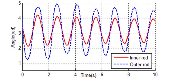
Table 4Some identification results of kinetic parameters with TGA

$G$	$m_{1}$	$m_{2}$	$m_{0}$	$l_{1}$	$l_{2}$	$J_{1}$	$J_{2}$	$c_{1}$	$c_{2}$	$H (Z)$
1	0.1296	0.1296	0.1622	0.288	0.14	0.0020	0.0018	0.00194	0.0035	73.512
20	0.1208	0.1144	0.1797	0.2743	0.149	0.0012	0.0017	0.00141	0.00331	11.9641
40	0.1036	0.1038	0.1622	0.2158	0.15	0.0009	0.0016	0.00378	0.0011	6.8701
60	0.1036	0.1049	0.1734	0.2132	0.15	0.0009	0.0015	0.00378	0.0007	3.5277
80	0.10350	0.10479	0.16323	0.22152	0.15	0.00070	0.00159	0.00378	0.00072	2.56147
100	0.10365	0.10529	0.16783	0.21121	0.15	0.00076	0.00159	0.00378	0.00066	2.48395
200	0.10365	0.10556	0.16745	0.20883	0.15	0.00069	0.00160	0.00387	0.00061	2.20321
300	0.10365	0.10552	0.16746	0.20828	0.15001	0.00069	0.00160	0.00388	0.00061	2.18617
400	0.10365	0.10552	0.16746	0.20671	0.15	0.00068	0.00160	0.00388	0.00061	2.17717
500	0.10374	0.10546	0.16746	0.20308	0.15	0.00066	0.00160	0.00392	0.00061	2.13894

4.2. Experimental results of traditional genetic algorithm

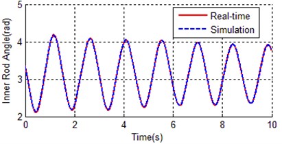
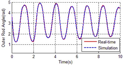
The chromosome is chosen as shown in Eq. (8), the solution space is defined by Eq. (9), and the fitness function is set up with Eq. (10). In all these cases, the traditional single point crossover is applied, the initial population is randomly generated, and the roulette selection operation is performed. Population size $M =$ 200, crossover rate $P c =$ 100 %, mutation rate $P m =$ 10 %, max generation is 500, and 4 steps of the Runge-Kutta method are adopted as a numerical algorithm, the step size is 0.005 s, the simulation duration is 10 seconds. Table 4 shows some identification results of kinetic parameters. Fig. 7 shows the evolutionary process of the best individual, and Fig. 7 shows the contrast curves of the inner and outer rods.

As it can be seen from Fig. 7, the convergence rate of traditional genetic algorithm is fast at the first 80 generations, the rest 420 generations tend to be stable, and the fitness of the best individual is 2.13894. There are totally 2000 data points, so the average error per point is 0.00106947, that is why the simulation curves (inner rod and outer rod) coincide with the reference trajectory shown in Fig. 8. The identification result of traditional genetic algorithm is much better than the estimated values in Table 2.

Fig. 7Evolution curve of best chromosome with TGA

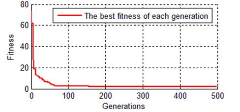
Fig. 8Contrast curves of real time and simulation for both a) inner rod and b) outer rod

a)

b)

4.3. Experimental results of improved genetic algorithm

Using the improved genetic algorithm mentioned in Section 3, the chromosome is shown in Eq. (9), the fitness function is shown in Eq. (10) and be further transformed with Eq. (7), population size $M =$ 200, crossover rate $P_{c} =$ 20 %, mutation rate $P_{m} =$ 2 %, max generation is 500. The IGA parameters are $α =$ 0.95, $σ =$ 5, $μ =$ 0.95, $ν =$ 0.10, $δ =$ 32. Simulation environment: 4 steps of the Runge-Kutta methodwith the step size of 0.005 s, simulation duration of 10s, Windows 10, Visual C++ 6.0.

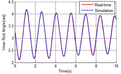
Table 5 shows some results of IGA, Fig. 9 shows the evolutionary process of the best chromosome. Fig. 10 shows the difference between simulation (with optimal kinetic parameters of IGA) and reference trajectory.

Table 5Some identification results of dynamic parameters with IGA

$G$	$m_{1}$	$m_{2}$	$m_{0}$	$l_{1}$	$l_{2}$	$J_{1}$	$J_{2}$	$c_{1}$	$c_{2}$	$H (Z)$
1	0.0921	0.1074	0.2449	0.2803	0.1659	0.0022	0.0014	0.0029	0.0068	90.802
20	0.1135	0.1044	0.1950	0.2648	0.1632	0.0009	0.0014	0.0032	0.0011	4.0011
40	0.1195	0.1046	0.1908	0.2608	0.1663	0.0008	0.0014	0.0033	0.0011	3.4501
60	0.1248	0.0960	0.1853	0.2526	0.1817	0.0007	0.0012	0.0042	0.0006	1.1053
80	0.1250	0.0976	0.1836	0.2541	0.1790	0.0007	0.0013	0.0042	0.0006	1.0658
100	0.1250	0.0976	0.1836	0.2541	0.1790	0.0007	0.0013	0.0042	0.0006	1.0658
200	0.1252	0.0982	0.1880	0.2481	0.1799	0.0007	0.0013	0.0043	0.0006	1.0057
300	0.1293	0.1009	0.1968	0.2377	0.1821	0.0007	0.0013	0.0046	0.0006	0.9271
400	0.1296	0.1151	0.2108	0.2186	0.1682	0.0007	0.0016	0.0049	0.0006	0.8629
500	0.1296	0.1154	0.2192	0.2007	0.1691	0.0007	0.0016	0.0049	0.0006	0.8515

Fig. 9Evolution curve of best chromosome with IGA

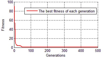
Fig. 10Contrast curves of real time and simulation for both a) inner rod and b) outer rod

a)

b)

As it can be seen from Table 5 and Fig. 9, the IGA tends to converge at about 70 generations, the fitness of the best chromosome is 0.8515, which is much better than the result of the traditional genetic algorithm (2.13894). This proved that the global searching ability of the improved genetic algorithm is better than the traditional genetic algorithm. Because the application of orthogonal experiments, the search efficiency of IGA has been greatly improved, this leads to the convergence rate of IGA faster than TGA. The error between simulation curves (with optimal parameters of IGA) and reference trajectory is so small (0.8515), that the curves almost overlapped as shown in Fig. 10.

4.4. Contrast between TGA and IGA

Both IGA and TGA achieved a remarkable improvement, the best individual of IGA is much better than TGA. Here we calculate the error between reference trajectory and simulation with optimal parameters for both TGA and IGA ( $θ_{i} (j) - {\hat{θ}}_{i} (j)$ ), Fig. 11 and Fig. 12 respectively show the angular error of inner rod and outer rod.

Fig. 11Angular error of inner rod between reference trajectory and simulation with optimal parameters

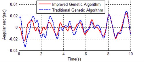
Fig. 12Angular error of outer rod between reference trajectory and simulation with optimal parameters

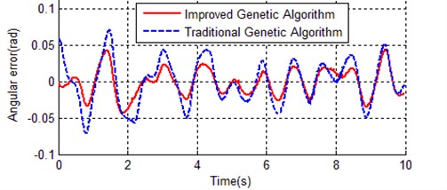
In Fig. 11 and Fig. 12, the vibration amplitude of dash line is obviously bigger than solid line in both Fig. 11 and Fig. 12, this means the optimal parameters obtained with the improved genetic algorithm is much closer to the actual device.

Fig. 13Contrast of evolution process of best individual between IGA and TGA

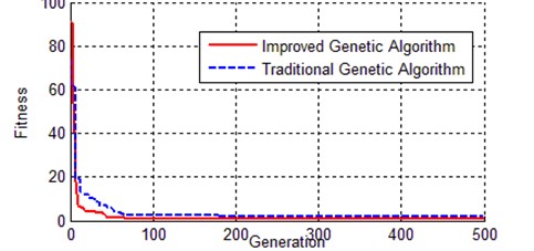
Fig. 13 shows the evolutionary process of the best chromosome for both the improved genetic algorithm and the traditional genetic algorithm. The TGA curve is always above the curve of IGA, which means IGA convergence faster than TGA, and the result of IGA is more accurate than that of the IGA.

5. Conclusions

An improved genetic algorithm is introduced to solve the problem of kinetic parameter identification for a cart double pendulum, which includes paring operation based on the hamming distance, variable precision crossover, orthogonal experiment, feedback mutation, and nonlinear transformation of the fitness function. The hamming distance guarantees the effectiveness of crossover operation. Variable precision crossover can search for a feasible solution from a low-precision to a high-precision solution space. Orthogonal experiment can find the optimal combination of parameters through fewer experiments. Feedback mutation fundamentally avoids the premature convergence of the genetic algorithm. Nonlinear transformation of the fitness function promotes the evolution to search the optimal generation. The error between the real-time response and simulation response as the fitness function, the contrast experimental results of empirical parameter, TGA optimized parameter, and IGA optimized parameter are provided. The result with IGA is obviously better than that with TGA and practical values, which verify the effectiveness of the proposed method.

References

Hung T. H., Yeh M. F., Lu H. C. PI-like fuzzy controller implementation for the inverted pendulum system. Proceedings of the IEEE International Conference on Intelligent Processing System, Beijing, China, 1997, p. 218-222.

Search CrossRef
Yang Yawei, Zhang Minglian Stability of numerical control of triple inverted pendulum. Journal of Beijing University of Aeronautics and Astronautics, Vol. 26, Issue 3, 2000, p. 311-314.

Search CrossRef
Li Hongxing, Miao Zhihong, Wang Jiayin Adaptive fuzzy control of fourfold inverted pendulum based on variable universe. Science in China (Series E), Vol. 32, Issue 1, 2002, p. 65-75.

Search CrossRef
Luis Alvarez Icaza Passivity-based swinging up of a pendulum. Proceedings of the 18th IFAC World Congress, Milano, Italy, 2011, p. 10667-10672.

Publisher
Pa Yee Tsai, Cha’o Kuang Chen Free vibration of the nonlinear pendulum using hybrid Laplace Adomian decomposition method. International Journal for Numerical Methods in Biomedical Engineering, Vol. 27, 2011, p. 262-272.

Publisher
Jian Huang, Zhi Hong Guan, Takayuki Matsuno, Toshio Fukuda, Kosuke Sekiyama Sliding-mode velocity control of mobile-wheeled inverted-pendulum systems. IEEE Transactions on Robotics, Vol. 26, Issue 4, 2010, p. 750-758.

Publisher
Li Zhijun, Luo Jun Adaptive robust dynamic balance and motion controls of mobile wheeled inverted pendulums. IEEE Transactions on Control Systems Technology, Vol. 17, Issue 1, 2009, p. 223-241.

Publisher
Li Z. S., Liang D. W. Human simulated intelligent controller with fuzzy online self-tuning of parameters and its application to a cart-double pendulum. Journal of Computers, Vol. 3, Issue 9, 2008, p. 67-76.

Publisher
Park M. S., Chwa D. Y. Swing-up and stabilization control of inverted-pendulum systems via coupled sliding-mode control method. IEEE Transactions on Industrial Electronics, Vol. 56, Issue 9, 2009, p. 3541-3555.

Publisher
Graichen K., Treuer M., Zeitz M. Swing-up of the double pendulum on a cart by feedforward and feedback control with experimental validation. Automatica, Vol. 43, Issue 1, 2007, p. 63-71.

Publisher
Li Zushu Zhou Qijian Ren Wei Identification of “quasi-equivalent” model and pade approximation with multi-adjustable parameters for dynamical systems. Acta Automatica Sinica, Vol. 11, Issue 1, 1985, p. 53-62.

Search CrossRef
Foster J. A. Evolutionary computation. Nature Reviews Genetics, Vol. 2, Issue 6, 2001, p. 428-436.

Publisher
Wu Mei, Lu Jingui Summary of research progress of genetic algorithms. Machine Tool and Hydraulics, Vol. 36, Issue 3, 2008, p. 176-179.

Search CrossRef
Li Zhushu, Tan Zhi, Wang Yuxin, Zhang Hua Real-time swing-up and handstand control of cart double pendulum on inclined rail. Proceedings of the 23rd Chinese Control Conference, Wuxi, China, 2004, p. 1645-1649.

Search CrossRef
Yin Wing Leung, Yuping Wang Orthogonal genetic algorithm with quantization numerical optimization. IEEE Transaction on Evolutionary Computation, Vol. 5, Issue 1, 2001, p. 41-53.

Publisher

Cited by

Study on Motion Control Problems for 3-DOF Underactuated Cart-Double Pendulum System

Lu Fan | Ancai Zhang | Xiao Liang | Xinghui Zhang | Jianlong Qiu

(2024)

Describing Droplet Motion on Surface-Textured Ratchet Tracks with an Inverted Double Pendulum Model

Mayssam Naji | Ecem Yelekli Kirici | Ali Javili | E. Yegan Erdem

(2021)

The control strength quantification analysis of outer pendulum rod for double inverted pendulum

Wencong Fu | Chan Wang | Peng Xu | Yuanhong Dan

(2019)

About this article

Received

17 March 2019

Accepted

10 June 2019

Published

30 September 2019

SUBJECTS

Mechanical vibrations and applications

DOI

https://doi.org/10.21595/jve.2019.20663

Keywords

cart-double pendulum

improved genetic algorithm

feedback mutation

variable precision crossover

Acknowledgements

This work was supported by the Chongqing Science and Technology Commission’s Technology Personnel Training Program (cstc2013kjrc-qnrc40010) and the Chongqing City Board of Education’s Science and Technology Research Project (KJ1709196).

This is an open access article distributed under the Creative Commons Attribution License, which permits unrestricted use, distribution, and reproduction in any medium, provided the original work is properly cited.

Previous article in issue Previous Next article in issue Next

Research article

2019 10 19

The control strength quantification analysis of outer pendulum rod for double inverted pendulum

Wencong Fu, Chan Wang, Peng Xu, Yuanhong Dan

Research article

2018 10 19

Optimization of critical speed of double spools with reverse rotation

Ze-gao Shi, Gui-huo Luo, Fei Wang

Research article

2018 02 15

Structural health monitoring of 3D frame structures using finite element modal analysis and genetic algorithm

S. Tiachacht, A. Bouazzouni, S. Khatir, A. Behtani, Y.-L.-M. Zhou, M. Abdel Wahab

Research article

2017 09 30

Precision prediction model in FDM by the combination of genetic algorithm and BP neural network algorithm

Hua Dong Yang, Sen Zhang

Y. Dan, P. Xu, W. Zhang, and Z. Tan, “Improved genetic algorithm for parameters identification of cart-double pendulum,” Journal of Vibroengineering, Vol. 21, No. 6, pp. 1587–1599, Sep. 2019, https://doi.org/10.21595/jve.2019.20663

Copy Extrica

Copied to clipboard!

TY  - JOUR
DO  - 10.21595/jve.2019.20663
UR  - https://doi.org/10.21595/jve.2019.20663
TI  - Improved genetic algorithm for parameters identification of cart-double pendulum
T2  - Journal of Vibroengineering
AU  - Xu, Peng
AU  - Dan, Yuanhong
AU  - Zhang, Wei
AU  - Tan, Zhi
PY  - 2019
DA  - 2019/09/30
PB  - JVE International Ltd.
SP  - 1587-1599
IS  - 6
VL  - 21
SN  - 1392-8716
SN  - 2538-8460
ER  - 

Copy Ris

Copied to clipboard!

@article{Xu_2019,
	doi = {10.21595/jve.2019.20663},
	url = {https://doi.org/10.21595/jve.2019.20663},
	year = 2019,
	month = {sep},
	publisher = {{JVE} International Ltd.},
	volume = {21},
	number = {6},
	pages = {1587--1599},
	author = {Peng Xu and Yuanhong Dan and Wei Zhang and Zhi Tan},
	title = {Improved genetic algorithm for parameters identification of cart-double pendulum},
	journal = {Journal of Vibroengineering}
}

Copy Bibtex

Copied to clipboard!

[1]P. Xu, Y. Dan, W. Zhang, and Z. Tan, “Improved genetic algorithm for parameters identification of cart-double pendulum,” Journal of Vibroengineering, vol. 21, no. 6, pp. 1587–1599, Sep. 2019, doi: 10.21595/jve.2019.20663.

Copy IEEE

Copied to clipboard!

Xu, Peng, Yuanhong Dan, Wei Zhang, and Zhi Tan. “Improved Genetic Algorithm for Parameters Identification of Cart-Double Pendulum.” Journal of Vibroengineering 21, no. 6 (September 30, 2019): 1587–99. https://doi.org/10.21595/jve.2019.20663.

Copy Chicago

Copied to clipboard!

Improved genetic algorithm for parameters identification of cart-double pendulum

Abstract

1. Introduction

2. Physical structure and mathematic model of cart double pendulum

3. Improved genetic algorithm

3.1. Pairing operation based on Hamming distance

3.2. Variable precision crossover

3.3. Orthogonal experiments in crossover operation

3.4. Feedback mutation

3.5. Nonlinear transformation of fitness function

3.6. Process of improved genetic algorithm

4. Experimental results

4.1. Chromosome and fitness function

4.2. Experimental results of traditional genetic algorithm

4.3. Experimental results of improved genetic algorithm

4.4. Contrast between TGA and IGA

5. Conclusions

References

Cited by

About this article

Related Articles