Abstract
This paper presents a vibration reducing mechanism combining the bi-directional evolutionary structural optimization (BESO) method and the multiple mass damper (MMD) method. The BESO method changes the mass and stiffness distribution of a structure, in order to push the most significant natural frequency away from the driving frequency. The removal of less stressed material by the BESO method creates hollow spaces in the structure. The MMD will be installed in the hollow spaces, and reduces the resonance vibration amplitude of the most significant mode.
1. Introduction
A structure on which a harmonic force of a constant frequency is acting may take up obnoxious vibrations, especially when the excitation frequency is close to a resonance frequency. In order to reduce such vibrations, we could first try to reduce the excitation force, but quite often it is not practical. Alternatively, we may change the mass and the stiffness of the structure. Another possibility is to use auxiliary systems like the tuned mass damper (TMD), invented by Frahm in 1911 [1, 2].
The structural optimization (SO) seeks to achieve the best performance for a structure while satisfying various constraints such as a given maximum amount of material [3]. In terms of computational effort, the BESO method is one of the most efficient SO methods [4]. It could be used to change the mass and the stiffness distribution, thereby increases the distance between the most significant natural frequency and the excitation frequency. This will reduce the resonance phenomena [5]. The single-degree-of-freedom (SDOF) TMD has been widely used to increase the performance of machining operations due to their simplicity, low cost and reliability [6]. However, the SDOF TMD is very sensitive to the natural frequency of the primary structure [7]. Therefore, its mistuning effect and narrow effective frequency band severely limit wider applications in engineering [7]. In order to solve these drawbacks, the MMD has been proposed [8]. In this paper, we combine the BESO method and the MMD method to reduce the vibration of a mechanical structure under a single external harmonic loading. The BESO method pushes the most significant natural frequency away from the driving frequency [5]. By removing less stressed material, the BESO method creates a hollow space, in which the MMD can be placed. The organization of the paper is as follows: in Section 2, we clarify the combination of the BESO method and the MMD method. We show the effectiveness of the combined mechanism with two numerical examples in Section 3. Conclusions from this study are presented in Section 4.
2. The combination of the BESO method and the MMD method
2.1. The BESO method with an adaptive filter scheme
The basic idea of the BESO method is to remove the unnecessary material from the structure [4]. Most of all, the BESO is a hard kill method, which means one element can only be solid or void [5]. This property can cause a serious problem: sometimes it removes elements, which transmit external loads into the structure [5]. In order to avoid this problem, we have proposed a filter scheme for the sensitivity number in [5]:
where , and are the von Mises stress for the -th element, the maximum of von Mises stress, and the normalized von Mises stress for the -th element in the static simulation. , and are the von Mises stress for the -th element, the maximum of von Mises stress and the normalized von Mises stress for the -th element in the dynamics simulation. is the sensitivity number for -th element, is the weighting factor of the static simulation, is the weighting factor of the dynamics simulation, is the distance between the centroid of the -th element and the load point, and p is the distance penalty factor. [5]
An optimal parameter set () of the filter scheme should fulfill two requirements. Elements in the load region will not be removed. And if or decreases, at least one of elements in the load region will be removed, which means the influence of the dynamic simulation has been considered to the maximum possible extent. There are many parameter sets, which fulfill the aforementioned requirements. But it is very difficult to find them before the BESO process. We can only improve the parameter set after a total BESO process and apply it to the next BESO process. The improvement process is very time consuming. Additionally, these optimal parameters are only optimal for the total BESO process, but not for each iteration of the BESO process. We must make a compromise here, either we choose and larger than necessary, in order to prevent the removal of elements in the load region. Or we choose a small and risking that the BESO process fails because of the removal of elements in the load region.
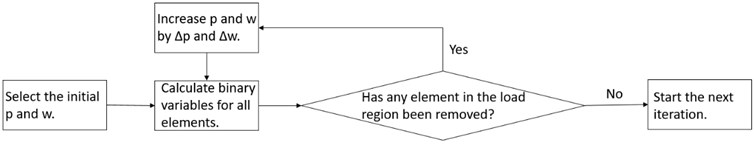
In order to solve the aforementioned contradiction, we upgrade the filter scheme to an adaptive filter scheme as shown in Fig. 1. We use very small initial and (e.g. 0). After the calculation of binary variables for all elements, we check if load region elements have been removed. If not, we go to the next iteration. If any element has been removed, we increase p and w and calculate binary variables again, until no load region elements have been deleted. With this adaptive filter scheme, we can have optimal p and w for each iteration.
Fig. 1The workflow of the adaptive filter scheme
2.2. The detection of internal nodes
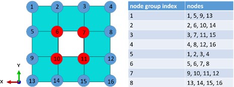
Before we mount the MMD into the FEM model of a structure, we should find potential mounting positions. Nodes on the surface of a FEM model could be classified into two subclasses, which are external surface nodes and internal surface nodes. All surface nodes could be mounting positions, but in order to reduce the occupied space of the structure, we prefer to choose internal surface nodes. A 2D FEM mesh is shown in Fig. 2. We can intuitively find out, that red nodes are internal surface nodes. But we need to describe internal surface nodes mathematically for complicated FEM meshes. We take the mesh in Fig. 2 as an example.
We build 8 groups of nodes as shown in Fig. 2. Each group has 4 nodes. In groups 1, 2, 3 and 4, all nodes in each group have the same coordinate, we name it common coordinate (CC), and a different coordinate, we name it non-common coordinate (NC). In groups 5, 6, 7 and 8, the coordinate is the CC, and the coordinate is the NC. We define the maximal NC value in each group as the upper limit (UL), the minimal NC value in each group as the lower limit (LL). Each node is a child node of two groups. If the NC value of the node is neither the UL, nor the LL in all of its parent groups, then we define this node as an internal surface node.
We expand this algorithm for 3D meshes. Each surface node has three parent groups, each group has 2 CC and one NC. If the NC value of one node is neither UL nor LL in all of its parent groups, it is an internal surface node.
Fig. 2A simple 2D FEM mesh
2.3. The installation of the MMD
After the BESO process and the detection of internal nodes, we are ready to install MMD into the structure. At first, we reduce the structure to an equivalent vibration system using the pseudo-kinetic energy approach (PKE). Then we tune the MMD based on the reduced system. At last we identify optimal mounting positions and mount the MMD automatically [9].
3. Numerical examples
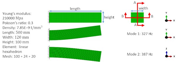
We present two numerical examples to show the effect of the combined vibration reducing mechanism. Both numerical examples considered the same traditional 3D cantilever beam as shown in Fig. 3. The target volume was 61 % of the design domain. We calculated the vibration amplitude at the load point in the mode-based steady state dynamics analysis, which considered all modes with natural frequencies lower than 7000 Hz in these two examples. We set initial filter scheme parameters () as (0, 0.02). In these two examples was fixed to 0 during the total BESO process, changed adaptively in each iteration. The first two modes before the optimization process are shown in Fig. 3.
Fig. 3The cantilever beam
3.1. Example 1
An external harmonic load with an amplitude of 1000 N and a driving frequency of 320 Hz excited the beam at the middle point of the right end in -direction. This frequency was near the first natural frequency 327 Hz. The objective of this example was to minimize the vibration amplitude of the load point in -direction at the driving frequency of 320 Hz, and at the same time to reduce the resonance amplitude of the first mode. We started the BESO process (from the number 0 to the number 39) first. Fig. 4(a) shows the evolutionary history of the weighting factor of the dynamics simulation. As a general tendency, it decreased slowly, in order to prevent the removal of elements in the load region. As shown in Fig. 4(b), generally the first natural frequency increased after each model update, which means it was pushed away from the driving frequency 320 Hz. But it could not always be increased at the same time of the removal of material, for example, the first natural frequency decreased in the iteration 39. As shown in Fig. 4(c), as the result of the increased distance between the driving frequency and the first natural frequency, the displacement of the load point under the harmonic excitation with the driving frequency decreased after each iteration. Fig. 4(e) shows FRFs of the cantilever beam, we can get the same conclusion as from the Fig. 4(b), the first natural frequency increased during the BESO process. The Fig. 4(d) shows the evolutionary history of the volume fraction. From iteration 1 to iteration 39, each iteration removed 1 % of material of the original model. The BESO process stopped after the iteration 39, because the target volume fraction 61% has been achieved. As shown in Fig. 5(a), a hollow space has been created during the BESO process. In iteration 40 we detected internal surface nodes and installed the MMD.
Fig. 4a) The weighting factor of the dynamics simulation, b) the first natural frequency, c) the displacement of the load point at 320 Hz, d) the volume fraction, e) FRFs
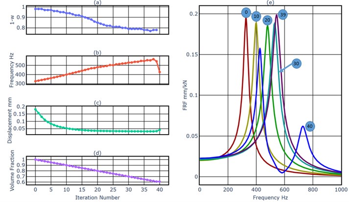
Fig. 5a) FEM models and their cross sections A-A as shown in Fig. 3, b) internal nodes at iteration 40, c) the installation of the MMD
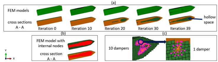
A one stage MMD with the mass ratio 5 % was installed into the structure during iteration 40. Fig. 5(b) shows detected internal surface nodes and Fig. 5(c) shows 10 masses of the MMD. The MMD was mounted at the unsupported side of the cantilever beam, because these nodes vibrated stronger than nodes close to the fixture. As aforementioned, the peak amplitude of the first mode should be reduced, so the MMD was tuned with the first mode as the target mode. Fig. 4(e) shows that, the first mode in iteration 39 was replaced by two modes during iteration 40. Even if we use the max value of peak amplitudes of two new modes as the indicator, the reduction of the peak amplitude of the first mode was still 19.4 %. Because the new first mode was pushed closer to the driving frequency of 320 Hz as shown in Fig. 5(b) and (e), the vibration amplitude at 320 Hz after iteration 40 is higher than in iteration 39. But the reduction of the vibration amplitude at 320 Hz after the combination process still reached 77.3 %.
3.2. Example 2
The second example is similar to the first one. The external harmonic load with an amplitude of 1000 N excited the beam at the middle point of the right end with a driving frequency of 380 Hz in -direction. This frequency was near the second natural frequency of 387 Hz. The objective of this example was to minimize the vibration amplitude of the load point in -direction at the driving frequency 380 Hz, and at the same time to reduce the resonance amplitude of the second mode as shown in Fig. 3.
Fig. 6a) The weighting factor of the dynamics simulation, b) the first natural frequency, c) the displacement of the load point at 380 Hz, d) the volume fraction, e) FRFs
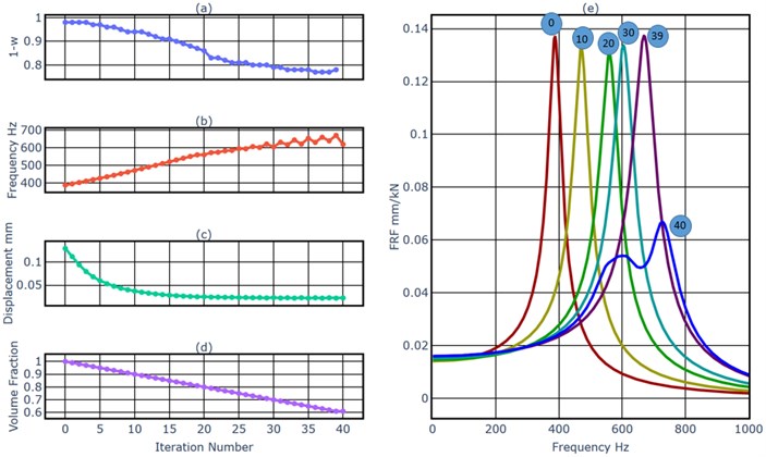
Fig. 7a) FEM models and their cross sections B-B as shown in Fig. 3, b) Internal nodes at iteration 40, c) The installation of the MMD
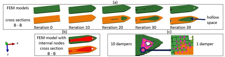
Fig. 6 and Fig. 7 show the result of the combination mechanism. As a general tendency, the decreased slowly, in order to prevent the removal of elements in the load region. The second natural frequency has been pushed away from the driving frequency as shown in Fig. 6(b). As shown in Fig. 6(c), as the result of the increased distance between the driving frequency and the second natural frequency, the displacement of the load point under the harmonic excitation with the driving frequency decreased after each iteration from iteration 0 to iteration 39. Fig. 7 shows detected internal nodes and 10 individual masses of the one stage MMD with a mass ratio 5 %. The MMD was mounted at the unsupported side of the cantilever beam, because nodes at the right side vibrated stronger than nodes close to the fixture.
As shown in Fig. 6(e), even if we use the max value of peak amplitudes of two new modes as indicator, the reduction of the peak amplitude of the first mode was still 51.1 %. The reduction of the vibration amplitude at 380 Hz after the combination process reached 82.2 %.
4. Conclusions
This paper presents a combined vibration reducing mechanism using the BESO method and the MMD method. The adaptive filter scheme of the BESO method selects optimal filter scheme parameters for each iteration, which prevent the removal of load region elements and considers the dynamic effect at the most possible extent in each iteration of the BESO process. The BESO process pushes the most significant natural frequency effectively away from the driving frequency, thereby it reduces the vibration amplitude of the load point at the driving frequency. The algorithm for the detection of internal nodes detects internal nodes after the BESO process, on which the MMD should be installed. The mounted MMD reduces the resonance vibration amplitude of the most significant mode effectively. The effectiveness of the combined vibration reducing mechanism has only been proven with FEM simulations. The designed structure with this combined vibration reducing mechanism could be manufactured with the 3D print technique. It could be used to mitigate the vibration at critical positions of machines, such as tool center points of machine tools.
As shown in Fig. 6(b), the most significant natural frequency increased with an oscillation. The possible reason is the numerical instability of the BESO process. As shown in Fig. 4(e) and Fig. 6(e), the effectiveness of MMDs for two examples was very different. We will find out reasons for these phenomena in the future. We will investigate the performance of the MMD produced with the 3D print technique. Thereafter we will validate the combined vibration reducing mechanism with a physical prototype.
References
-
Den Hartog J. P. Mechanical Vibrations. Dover Edition, Dover Publication Inc., New York, 1985.
-
Frahm H. Device for Damping Vibrations of Bodies. United States Patent 989,958, 1911.
-
Huang X., Xie M. Evolutionary Topology Optimization of Continuum Structures. Methods and applications. John Wiley and Sons, 2010.
-
Huang X., Xie M. Convergent and mesh-independent solutions for the bi-directional evolutionary structural optimization method. Finite Elements in Analysis and Design, 2007.
-
Brecher C., Zhao G., Fey M. Topology optimization for vibrating structures with the BESO method. Vibroengineering Procedia, Vol. 23, 2019, p. 1-6.
-
Munoa J., et al. Chatter suppression techniques in metal cutting. CIRP Annals, Vol. 65, Issue 2, 2016, p. 785-808.
-
Dai J., Xu Z., Gai P. Dynamic analysis of viscoelastic tuned mass damper system under harmonic excitation. Journal of Vibration and Control, Vol. 25, 11, p. 1768-1779.
-
Xu K., Igusa T. Dynamic characteristics of multiple substructures with closely spaced frequencies. Earthquake Engineering and Structural Dynamics Vol. 21, Issue 12, 1992.
-
Schmidt S. Distributed Multi-Mass Dampers for Machine Tools. First Edition, Apprimus, Aachen, 2019.
About this article

The authors would like to thank the German Research Foundation (DFG) for supporting this research under Grant No. BR2905/57-3: “Optimale Positionierung und Auslegung von Mehrmassendämpfern innerhalb eines kombinierten Topologieoptimierungsverfahrens”.
