Abstract
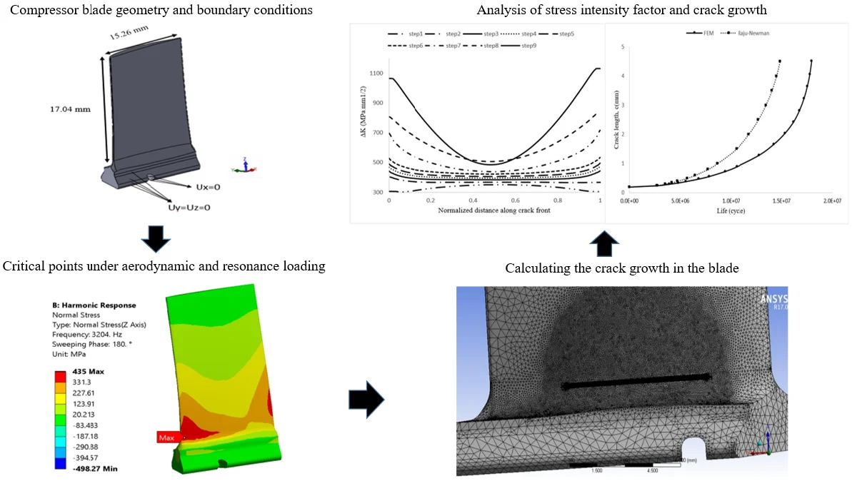
In this study, the cracks growth rate in the 13th row of the T56 compressor blades was studied to investigate their fatigue life. For this purpose, the centrifugal and aerodynamic forces on the blade were calculated and then the resulting stress field was obtained by using finite element method. Then, the critical points of stress were determined and the initial semi-elliptical cracks were modeled at these points. After modeling of the initial crack, the stress intensity factor on the crack front was calculated by ANSYS software. Furthermore, the number of required cycles for the crack growth and blade fracture were calculated by applying Paris law to a certain value. After crack growth at this stage, a crack with new length was also modeled at the same point and all the mentioned stages for its growth, were repeated. In this paper, the modal analysis of the blade was conducted and normal frequencies with possible stimulation on compressor velocity were determined by Campbell Diagram. After determining the stress field at resonant frequency, all stages of crack growth were repeated under these conditions to calculate the fatigue life.
Highlights
- Calculation of fatigue life for a compressor blade using Paris law, finite element analysis and computational fluid dynamic
- Analysis of the blade under both aerodynamic and resonance loading condition
- Determining and comparison the crack growth pace and direction in all of the steps
1. Introduction
Compressor blades are exposed to high rotational velocity in low temperature and hence undergo high centrifugal forces which can cause different kinds of problems from which nucleation and growth of cracks can be named [1]. Therefore, the blades should be designed in a perfectly safe manner, since the blade stall or break can disrupt the entire engine performance. The initiation or propagation of cracks in a blade stems from three major phenomenon namely: flaws in the material, stress concentration zone and fretting wear due to contact between two materials.
Novel studies have been conducted on replacement of new materials including composite and intermetallic [2-5]. Various studies have concentrated on fatigue life prediction of materials with different properties by both analytical [6-8] and experimental [9-11] methods. In 1985, Broek announced that there probably exist as many equation to predict fatigue life of a material under particular condition of experiment so there is no ethical equation which fill all data of different crack kinds [12]. Newly studies have considered composite materials in order to compare their functionality under high cycle fatigue load (HCFL) wherein turned out the fatigue functionality of composite materials to be better than isotropic ones [13-16]. Although replacement of newly materials in order to promote the fatigue life of structures are now well extended, these materials are expensive to manufacture and so one need to introduce an applicable method.
Analysis of fatigue performance in any part can be viewed in two different aspects namely: calculation of life in an intact model of the part and analysis of the model assuming the existence of an initial defect which usually will be considered at the stress concentration area in the model [17]. Witek in a study showed in model without initial defects, crack will nucleate from the bottom of the convex of the blades [18]. Life prediction of materials has been calculated by using failure Analysis Methods [19-21] and implementing experimental analysis to evaluate the failure and identify the effective factors on blades stall [22-24]. Optimization of geometrical and manufacturing parameters in a model by FE methods have the objective of various studies [25-27]. Gianella et al in 2018 investigated a fatigue fracture assessment utilizing an uncracked part from which output results were used as input for the final cracked model simulation. In aforementioned research a quarter-ellipse corner crack was considered as a defect in the model [28].
In this research the position and size of the initial crack in a fractured blade was determined using finite element analysis under fracture circumstances, and the stress field on the blade was calculated. The propagation procedure of the crack was conducted by using ANSYS software to calculate stress intensity factor and Paris Law to determine required cycles for crack growth. The analysis was conducted in three different positions and for 17 growth stages. Modal analysis of the model were carried out and normal frequencies with possible stimulation on compressor velocity were determined by Campbell Diagram. In the final stage of the study all the crack growth steps were carried out using stress field at resonant frequencies.
2. Materials and geometry
The considered engine is a 14-row compressor and its turbine consists four rows of blades. Other technical specifications are listed in Table 1.
The blade row examined in this study is fabricated from stainless steel 17-4PH (H1100). The constituent elements and mechanical properties of this alloy are listed in Tables 2 and 3, respectively. The steel is heated to the temperature of 1100 °F under annealing operation and cooled down in the air.
Table 1Technical specifications of the engine
Inflow mass discharge (kg/s) | Compression ratio | Rotational velocity (rpm) | Turbine input temperature (C) | Output power (Kw) | Mass (Kg) | Diameter (m) | Length (m) | Type |
14.5 | 2.25:1 | 13820 | 860 | 3915 | 880 | 0.69 | 3.7 | turboprop |
Table 2Chemical composition of H1100 alloy [29]
Iron | Carbon | Titanium | Manganese | Silicone | 17-4 PH cooper | Nickel | Chrome |
Balance | 0.07 % | 0.15-0.45 % | 1 % | 1 % | 3-5 % | 3-5 % | 15 % |
Table 3Mechanical properties of steel alloy (H1100) PH 17-4 [29]
Fracture toughness | Elongation at fracture (%) | Poisson ratio | Final stress (MPa) | Yield stress (MPa) | Elasticity Module (GPa) | Density (g/cc) |
2055 | 14 | 0.272 | 965 | 793 | 204 | 7.815 |
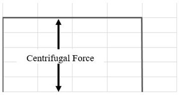
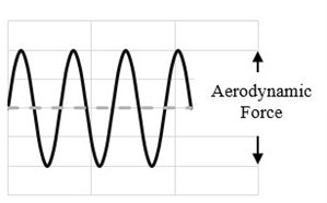
The most important forces on compressor blades are centrifugal force due to rotational velocity, and aerodynamic force due to collision of the inlet air to the blades. The centrifugal force applies as a constant tensile stress force and aerodynamic force applies as an oscillating bending stress force on blades.
3. Finite element stress analysis
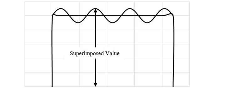
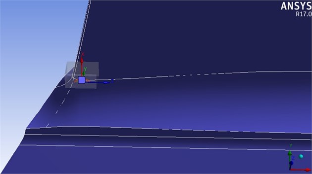
The blades are under a cyclic loading in which the centrifugal force plays a moderate role and the aerodynamic force determines the amplitude of the oscillation of the applied stress. Therefore, in order to demonstrate the total loading considering Fig. 1, a procedure of superimposition is applied in which a major mean stress arising from centrifugal forces and a cyclic variation arising from aerodynamic forces are affecting the model simultaneously. Boundary conditions of displacement applied to the blade are also shown in Fig. 2.
The ANSYS17 finite element software was used to calculate the stress field caused by the forces mentioned above. For this purpose, after real-dimensional 3D scanning, the blade was modeled in SOLIDWORKS software, as shown in Fig. 2, and then the model was exported– to the finite element software for analysis. The finite element model was created using 85608 elements of 10 nodes Solid 187.
Fig. 1Schematic diagram of fatigue loading applied to the compressor blades: a) mean stress caused by centrifugal force, b) cyclic stress caused by aerodynamic force, c) superimposition of two loads
a)
b)
c)
Fig. 2Boundary conditions of displacement applied to the blade
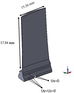
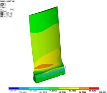
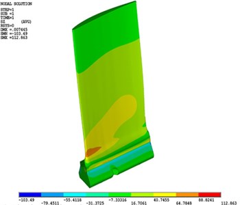
The static normal stress field on the blade due to rotational velocity of 13820 rpm and rotational radius of 165 mm and mass of 3.59 gr on both pressure and suction sides is shown in Fig. 3. One could see that the maximum normal stress happens in the scape edge of the blade.
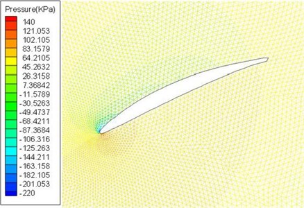
On the other hand, to calculate the air pressure on the blade, the blade airfoil was sketched in Fluent Software. Then, as it could be shown in Fig. 4, the pressure field around it was calculated by applying velocity triangles in input and output of the blade.
Fig. 3Normal stress (σzt) distribution caused by centrifugal force on the: a) suction surface and b) pressure side
a)
b)
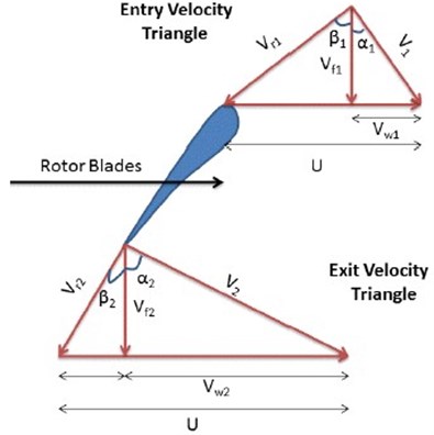
To apply boundary conditions in simulation, the velocities of (air absolute velocity) and U (linear velocity of the blade) were applied on inflow air and blade based on provided velocity triangle in Fig. 4. The static pressure distribution results on the airfoil area are shown in Fig. 5. As it can be seen, the average difference of the pressure and suction sides is about 60 KPa.
Fig. 4Entry and exit velocity triangles of the blade
The pressure field caused by aerodynamic forces could be driven for verifying the results from turbo-machine relations.
In Fig. 4, is the axial velocity of air, is the linear velocity of blade, is the relative velocity of air, is the absolute velocity of air, is the tangential velocity of air, is the angle between air relative velocity and axial direction, and is the angle between air absolute velocity and axial direction:
In previous Eq. (1), is the transient mass flow rate on the blade:
Based on Fig. 3 and 4, the necessary inputs to calculate the velocities of and are as follows:
By assuming that the input inflow is axial, we have , and due to the geometry of the blade 12.54°; as a result, we have:
Consequently, resultant force can be driven from Eq. (1) equal to 13/12N. Finally, aerodynamic pressure could be driven by divide force by pressure area which is 260 mm2:
So, one could say that calculation of air pressure which was provided in the previous section, presents reasonable answers.
In order to obtain the stress field due to aerodynamic pressure (Fig. 5), pressure difference between the pressure and suction sides was determined based on Fig. 6; as well as, the pressure distribution equation based on parameter “” was obtained by fitting a 6-order equation on each of them. As it can be seen in Fig. 6, the aerodynamic pressure based on the resulted equation was applied on both suction and pressure sides in ANSYS software.
Fig. 5The static pressure distribution produced by airflow around the airfoil
By applying the aerodynamic and centrifugal force simultaneously as shown in Fig. 7(a) and 7(b), in bending to the left, pressure side undergoes positive normal stress and suction surface undergoes negative normal stress. The adverse of this theory is also dominating in bending to the right. By considering bending stresses, in bending to the left, the maximum value occurs on the corner of pressure attack trailing edge where the kinetic energy is mostly emerged as pressure energy [21], and according to the contour results in bending to the right the maximum value of bending stress occurs in the middle of suction surface [30].
According to Fig. 7(a), the maximum value of normal stress on the pressure side is equal to 145 MPa and based on Fig. 7(b) the maximum value of normal stress on the suction surface is 140 MPa. These stress values are very low compared to blade yield point which is equal to 793 MPa. So, the blade is on a safe margin of design based on maximum stress. This condition has been also mentioned in the other studies that in the blades design, their lifetime was infinite due to finite applied stresses and the blades were always designed in a very safe area. However, a phenomena such as foreign object damage (FOD) or vibration resonance, which are largely inevitable, always obscure the safe design of blades. The foreign object damage creates small cracks in the blade surface. If these cracks are near critical points, they could grow rapidly and cause the blade to fail.
Fig. 6Pressure distribution on the pressure and suction sides of the blade
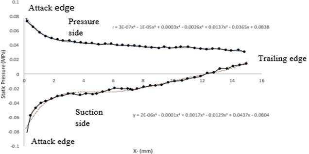
Fig. 7a) Normal stress (σz) distribution in bending to the right on normal stress suction side, b) normal stress (σz) distribution in bending to the left on pressure side due to centrifugal and aerodynamic force
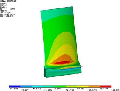
a)
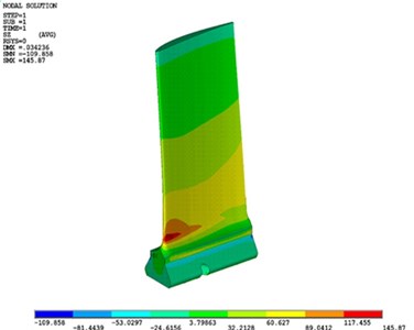
b)
4. Finite element model
As it is shown in the stress analysis results, the two points with maximum stress that are prone to crack formation are identifiable on the pressure and suction surfaces. The dimensions of initial cracks have been selected in such a way that the maximum value of stress intensity factor will be in the range of threshold stress intensity factor that is about . Therefore, semi elliptical crack was modeled based on Fig. 8 with a large diameter of 0.2 mm and a small diameter (depth) of 0.1 mm.
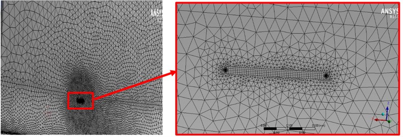
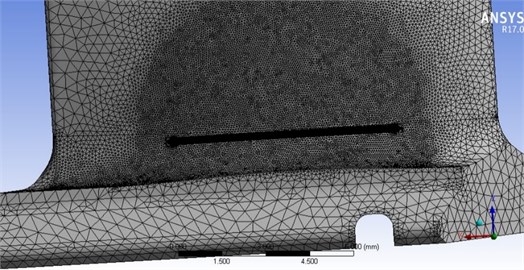
To mesh the cracked area, first, the initial crack front was divided into 60 seeds. With increasing crack’s length, these parts are increased. Moreover, in order to have preferred elements in the cracked area (Fig. 9), the software features were used to divide the spherical area with a radius of twice the length of the cracks (concentric with the crack) and the size of each element were equal to 0.05 mm. Now, after meshing the whole blade, as well as manual meshing the area around the crack, the geometry and finite element model of crack created on both the pressure and suction surfaces.
Fig. 8Position of the initial cracks: a) suction surface and b) pressure surface
a)
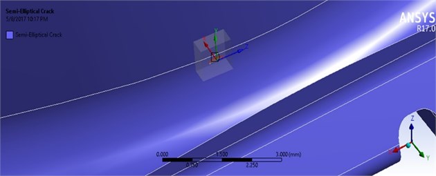
b)
Fig. 9Meshing the area around the crack
5. Results
5.1. Calculations of crack growth on the suction side
After modeling the initial crack on the pressure and suction surfaces and applying the mentioned forces on the blade, the stress intensity factor values on the crack front were calculated by the software. After determining the values of stress intensity factor; Paris law [31] is used to determine the crack growth. This equation is defined as follows:
In which, is the crack growth rate (increased crack length in one cycle), and C & n are the constants of Paris law. The constants C & n for different stress ratios are presented in Table 4.
is defined as follow:
In which, is the maximum stress intensity factor (SIF) in a loading cycle and is the minimum value. In the case of discrete crack propagation, the Paris law is as follows:
Table 4The Paris law constants C and n for stainless steel (H1100) 4-17 PH in different stress ratios [32]
Constants | 0.04 | 0.3 | 0.67 |
3.245 | 3.22 | 3.2 | |
4.96×10-¹⁴ | 1.12×10-¹³ | 2.52×10-¹³ |
The cracks growth path is calculated as follows: First, maximum and minimum stress intensity factor on the initial crack front is calculated and then the crack length () at 0° will be increased to a certain amount in each stage. Then using Paris law, the total number of required cycles for crack growth to obtain the value of will be calculated. After calculating the number of cycles by reusing Paris law, the value of increasing the length and are obtained at each stage. In Fig. 10, the parameters mentioned above are shown. It should be noted that and are different, given that the cracks do not grow symmetrically.
Fig. 10A view of crack shape and applied parameters
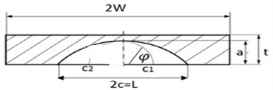
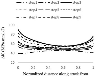
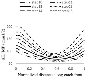
Fig. 11Distribution of stress intensity factor changes of crack front on the suction side during: a) steps 1 to 9 b) steps 10 to 15 of growth
a)
b)
Fig. 11 shows the stress intensity factor changes distribution within different stages of crack growth. At all stages except the first one, stress intensity factor at the point of 0° is greater than its value at the points of 90° and 180°. It means that the increase in the crack length is faster than its depth and also, the crack growths more toward attack edge (instead of trailing edge) [33]. The reason that this behavior is not observed in the first stage of growth is explained in [34] as follows: generally, semi elliptical cracks tend to change to semicircular cracks during the initial growth stages.
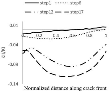
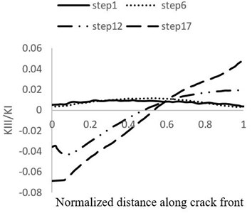
In Fig. 12, the stress intensity factor ratio of the second mode to the first mode ( and the stress intensity factor ratio of the third mode to the first mode ( during the growth stages are shown. It could be seen that the value of stress intensity factor in the second and third modes is negligible compared to the first mode. Therefore, this case could be simulated as pure first mode. Calculated stress intensity factors for each crack growth stage in points of Ø = 0°, 90°, 180° are shown in Table 5.
Fig. 12Comparison between KI and a) KII and b) KIII
a)
b)
Table 5Calculated stress intensity factors for each crack growth step in points of Ø = 0°, 90°, 180° on the crack front
Growth steps | ||||||
1 | 53 | 11.7 | 60 | 14.7 | 53 | 11.7 |
2 | 69.5 | 14.6 | 64.5 | 17.6 | 69.1 | 16.7 |
3 | 74.7 | 15.7 | 67.9 | 19.4 | 73.9 | 18.3 |
4 | 78.8 | 16.6 | 70.7 | 21.0 | 77.9 | 19.7 |
5 | 82.6 | 17.4 | 73.5 | 22.7 | 81.6 | 21.1 |
6 | 88.4 | 18.5 | 78.0 | 25.5 | 87.1 | 23.5 |
7 | 95.1 | 19.0 | 81.9 | 27.7 | 93.5 | 25.2 |
8 | 103.1 | 20.0 | 88.4 | 32.2 | 101.0 | 28.7 |
9 | 112.8 | 22.1 | 93.6 | 37.8 | 110.0 | 33.7 |
10 | 126.6 | 23.1 | 106.8 | 46.3 | 123.5 | 40.1 |
11 | 137.6 | 24.4 | 132.0 | 62.5 | 137.1 | 45.9 |
12 | 149.4 | 26.7 | 132.0 | 62.5 | 155.2 | 53.1 |
13 | 174.0 | 36.2 | 144.1 | 74.5 | 181.5 | 65.8 |
14 | 195.0 | 45.1 | 160.5 | 83.3 | 203.5 | 74.2 |
15 | 222.2 | 57.6 | 176.1 | 94.7 | 232.4 | 88.3 |
16 | 247.8 | 69.9 | 191.4 | 104.6 | 261.3 | 102.0 |
17 | 291.1 | 91.3 | 212.5 | 121.6 | 308.4 | 123.1 |
In Table 6, the crack length and depth are provided along with the number of required cycles in each grow stage.
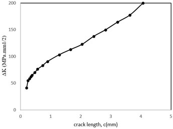
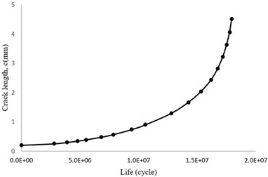
Stress intensity factor changes related to crack length are shown in Fig. 13. The crack depth to crack length ratio is also shown in Fig. 14. Furthermore, the stress ratio () changes and crack length diagram based on the number of cycles are shown in Fig. 15 and Fig. 16, respectively. Regarding Fig. 13, the variation of stress intensity factor versus crack length comprises three distinct stages: the initial stage shows an intense slope, but in the middle stage the slope decreases and for the final stage the slope of plot increases as similar as the first stage. Notably, plots revealed by Hu et al have similar stages [35].
Table 6Crack length and depth along with the number of required cycles in each grow stage
Grow stages | Crack length (mm) | Crack depth (mm) | (mm) | (mm) | (mm) | Cycles required for each growth stage () | Total number of cycles () |
1 | 0.2 | 0.1 | 0.05 | 0.05 | 0.067 | - | - |
2 | 0.25 | 0.167 | 0.05 | 0.043 | 0.030 | 2784203 | 2784203 |
3 | 0.297 | 0.197 | 0.05 | 0.041 | 0.027 | 1118431 | 3902634 |
4 | 0.342 | 0.224 | 0.05 | 0.040 | 0.024 | 888439.9 | 4791074 |
5 | 0.387 | 0.248 | 0.1 | 0.078 | 0.045 | 746380.5 | 5537454 |
6 | 0.476 | 0.293 | 0.1 | 0.074 | 0.040 | 1280825 | 6818279 |
7 | 0.563 | 0.332 | 0.2 | 0.141 | 0.067 | 1026326 | 7844605 |
8 | 0.734 | 0.399 | 0.2 | 0.128 | 0.057 | 1558762 | 9403367 |
9 | 0.898 | 0.456 | 0.5 | 0.287 | 0.118 | 1178061 | 10581429 |
10 | 1.292 | 0.574 | 0.5 | 0.249 | 0.088 | 2218404 | 12799833 |
11 | 1.666 | 0.663 | 0.5 | 0.249 | 0.104 | 1451238 | 14251071 |
12 | 2.041 | 0.767 | 0.5 | 0.277 | 0.080 | 1087807 | 15338878 |
13 | 2.429 | 0.847 | 0.5 | 0.285 | 0.055 | 839950.8 | 16178829 |
14 | 2.88 | 0.902 | 0.5 | 0.311 | 0.059 | 578054 | 16756883 |
15 | 3.227 | 0.961 | 0.5 | 0.327 | 0.052 | 439861.8 | 17196744 |
16 | 3.640 | 1.013 | 0.5 | 0.350 | 0.049 | 326137.1 | 17522882 |
17 | 4.065 | 1.063 | 0.5 | 0.392 | 0.040 | 253589 | 17776471 |
18 | 4.511 | 1.102 | - | - | - | 174437 | 17950908 |
Fig. 13Stress intensity factor changes related to the crack length
Based on the results showed by Nabavi et al for a constant value of stress intensity factor by increasing the value of crack length a decreasing trend in the aspect ratio would be obvious which is in a good accordance with results of Fig. 14, showing the tendency of the crack to change from an elliptical shape into a circular shape [33].
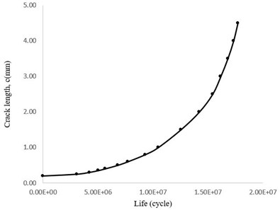
Considering Fig. 16 it can be seen that the blade fails after about 18×106 cycles. The graph shows also that the maximum loading time was spent for crack growth up to 2 mm. Poursaeidi et al have illustrated that in all analytical cases by the use of both Newman solution and weight function methods and also experimental cases for crack length greater than 4 mm the slope of c-N plot increases dramatically which is in a good accordance with the results illustrating in Fig. 16. Besides, the results are also in a good agreement about the predicted life cycles values [36]. It can be deduced that the blade life will be very short after the aforementioned stage and it will be failed quickly.
Fig. 14Aspect ratio (a/c) changes related to the crack length
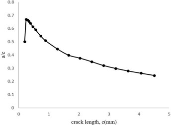
Fig. 15The stress ratio parameter changes with the crack length
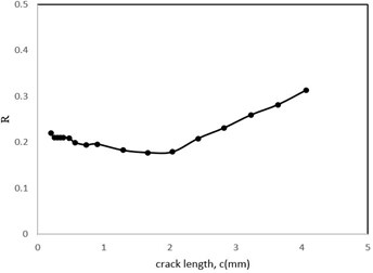
Fig. 16Crack length diagram versus total number of cycles (c-N)
To convert life per number of cycles to life per hours, the following equation is used:
where, is the number of cycles and 230 rev/s is the blade rotational velocity.
Finally, Fig. 17 is a view of modeled crack in the last stage of the growth simulation.
Fig. 17Simulated crack in the last growth stage
5.2. Raju-Newman solution for calculating stress intensity factor in a plate with semi-elliptical crack in order to verification
Raju and Newman [37] presented the following equation for calculating the first-mode stress intensity coefficient in a plate under tensile and bending stresses, including the semi elliptical crack, as shown in Fig. 18:
where is the coefficient of bending and and are tensile and bending stress, respectively. Besides, is the ellipse shape factor and is the boundary correction factor, which depends on crack depth, crack length, plate thickness, and plate width.
Fig. 18Crack and geometrical parameters in Raju-Newman solution [33]
![Crack and geometrical parameters in Raju-Newman solution [33]](https://static-01.extrica.com/articles/21092/21092-img25.jpg)
The assumption is intended to use the Raju-Newman equations to calculate the coefficient of stress in the blade in such a way that the section of the blade airfoil is considered as a rectangle and given that the cross-sectional area is 14.13 mm2 and the Camber is 15.26 mm, so the blade section is assumed to be a rectangle with dimensions of 15.26 mm×0.926 mm.
Calculated stress intensity factor from both solutions are shown in Fig. 19. In initial stages the results are in complete agreement and by reaching the crack size equal to 2 mm, the results differ a little with each other.
The results of crack growth rate obtained from Raju-Newman solution and the results obtained from the finite element method are shown in Fig. 20. For the small values of crack length, the two graphs coincide. In the following, with increase in the crack length, the two solutions are separated and at the last stage, the difference between the two methods is 17 %, which is due to the following:
A) Geometrical differences in the two solutions.
B) In the finite element model, the cracks length does not grow symmetrical in two directions (), and this causes the growth rate of the crack length to decrease compared to the Raju-Newman method.
Fig. 19Stress intensity factor variation with the crack length based on two solutions
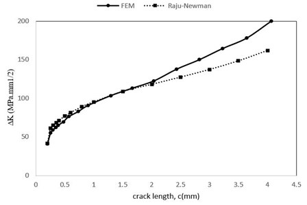
Fig. 20Crack length diagram versus total number of cycles (c-N)
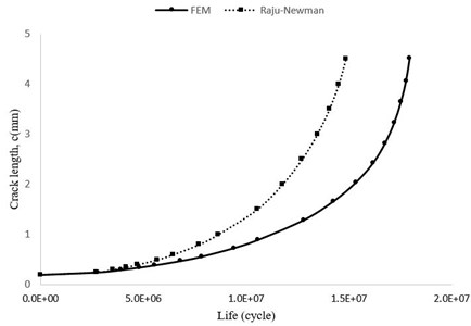
In the results of research [18] and [36] which was been used by the Raju-Newman method, it has been shown that the calculated lifetime of this method is less than the calculated lifetime of experimental and finite element modeling.
5.3. Calculations of crack growth on the pressure side
The simulation steps and the crack growth process are similar to Section 5-1, except that the crack on the pressure side after the first stage of growth has reached the edge of the attack, and thus the behavior of the crack is similar to that of the left-handed behavior. This means that the large diameter of the crack (the crack length) in this case will grow only in one direction (∅ = 0) and towards the trialing edge. Variations of the maximum stress intensity factor with the crack length and the crack growth rate graph are shown in Fig. 21 and Fig. 22, respectively. The description of these shapes is similar to Fig. 11 and Fig. 16, which is why their descriptions are ignored.
5.4. Campbell diagram
The Campbell diagram is used to study the probability of resonance phenomenon in turbines and compressors. In this diagram, various modes of the blade natural frequency are obtained using experimental methods and/or the finite element method simulations and turbine resonant frequencies are plotted against each other; so that, the probability of occurrence of the resonance phenomenon in various modes near the correct coefficients of a number of fixed compressor blades are studied. The first stimulation frequency should be plotted according to acceleration lines of API-612 [35] up to fifteenth factor.
Fig. 21Stress intensity factor variations related to crack length
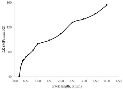
Fig. 22Stress intensity factor variation based on tow solutions with crack length
The second group of stimulation frequencies are related to the number of nozzles. The third group is partial suction frequency of the nozzles; which may cause a small amount of stimulation and this stimulation depends on the number and spacing of nozzles. It can be ignored to simplify the problem.
The blade stimulation frequency depends on the number of fixed blades and rotor rotation velocity. To analyze the results, the modes shapes were plotted in resonant line-harmonic intensity (Campbell diagram). Harmonic stimulation is considered as a fixed number of blades. The intensity line is defined as the nozzle passes the frequency.
In this compressor and considering the fact that the number of nozzles in the thirteenth and twelfth row is 96 and 75, respectively, then, nuzzles stimulation frequency can be calculated by the following relation:
– Number of rotor rotations per second × Number of nuzzles per row = Nozzle stimulation frequency
– Stimulation frequency of nozzles in the thirteenth row = 230×95 = 21850 Hz.
– Stimulation frequency of nozzles in the twelfth row = 230×75 = 18400 Hz.
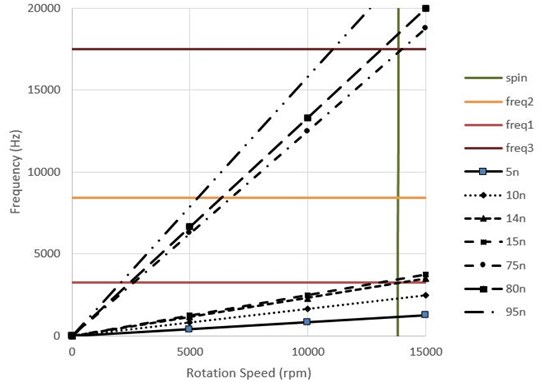
The corresponding Campbell Diagram has been plotted in Fig. 23. It can be seen that in the fourteenth stimulation in a working cycle; the compressor exacerbates the stimulation in the first vibrational mode and then, the seventy-fifth stimulation of nuzzles in the twelfth row exacerbates the third vibrational mode.
Fig. 23Campbell diagram for 13820 rpm
5.5. Harmonic analysis
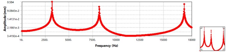
The results of the modal analysis which shows first three natural frequencies as: 3241, 8406 and 17514 Hz, respectively; were linked to the software harmonic analysis section and then the harmonic analysis was carried out by applying the aerodynamic pressure on the blade in the frequency range of 0-18000 Hz with a constant damping coefficient of 0.006. The frequency response of the blade is shown in Fig. 24. Three peaks formed in Fig. 24 are related to the natural frequencies displacement of the blade.
Fig. 24Frequency response of the blade
5.6. Stress analysis in the first natural frequency
Regarding the probability of occurrence of the first and third resonance blade frequency in the compressor operation, the stress field is determined by applying aerodynamic load with frequencies equal to the first and third modes of frequency, and critical points that are more likely to be cracked, are detected. Since the third natural frequency is very high and the probability of occurrence is less than the first natural frequency, the above-mentioned cases are only performed at the first natural frequency.
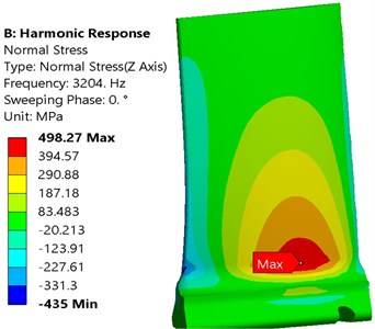
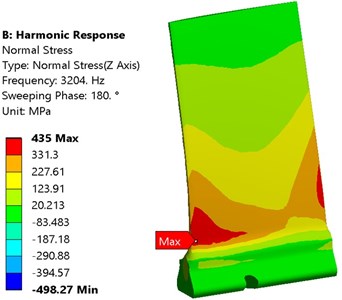
The first peak in Fig. 25 is related to the first natural frequency which is 3204 Hz. In order to determine the stress field, aerodynamic pressure with frequency of 3204 Hz was applied on the blade. In Fig. 25(a) and (b), normal stress field was applied on both the suction and pressure surfaces at angles 0° and 180°, respectively.
To calculate the blade life in the natural frequency of the first mode, a similar approach to the previous section was applied; so that, the initial semi elliptical crack with the length of and depth of was modeled in the critical point and it grew in 9 stages.
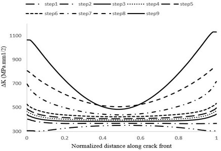
After crack modeling and its step by step growth, the results related to stress intensity factor distribution is shown in Fig. 26. Distribution of the stress intensity factor is similar to the crack on the suction surface which previously described. However, in the case of intensity, the stress intensity factor value is much higher.
Fig. 25Normal stress (σz) distribution in the first natural frequency: a) suction and b) pressure surface
a)
b)
Fig. 26Maximum stress intensity factor distribution variations at different stages of crack growth
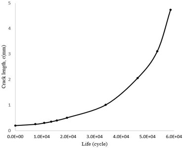
In Fig. 27, stress intensity factor variations versus crack length are shown. It is also observed that increased rate of is very high in the initial growth stages, and hence, it will decrease after a while. On the other hand, it can be seen in Fig. 28 that most of the applied cycles cause length increase up to 1mm and then, the crack continues to grow fast. After about 30,000 cycles, the crack length reaches 1 mm and after 60,000 cycles it reaches a length of 4.7 mm, in which the crack growth rate is high and the blade fails quickly.
Fig. 27The stress intensity factor variations during increasing cracks length
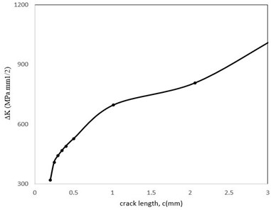
Fig. 28Crack growth rate (c-N)
6. Conclusions
The aim of this study was to numerically analysis a compressor blade fatigue life under the presence of both aerodynamic and centrifugal forces using finite element analysis and computational fluid dynamic method. By applying calculated forces from the Fluent Software on the blade, stress field of each of them was obtained by ANSYS Software. Using the stress contours the critical points on both pressure and suction surfaces of the blade were determined. The stress analysis results also showed that the stress field resulted from the centrifugal and aerodynamic forces were much less than the yield strength and fatigue limit endurance of the blade. Therefore, accordance to literature of the subject, foreign factors, such as corrosion, foreign objects damage, or vibration resonance phenomena gave rise to the formation of initial cracks in the blade. In order to calculate the fatigue life, initial semi elliptical crack was implemented in each of the aforementioned points. Besides, stress results were applied into the Paris law in order to simulate the crack growth rate. Furthermore, by reaching the crack growth to a certain value according to the Paris law, a new crack with a new length was created on the blade and all the aforementioned steps were repeated for this new crack. This procedure continued until the last stage of growth. In this way, fatigue life of the blade along with the crack growth rate was determined by cracking on both the suction and pressure surfaces. The most prominent results are as follows:
1) The maximum stress value in the blade bending to the left, occurs on the corner of pressure attack trailing edge, where the kinetic energy is mostly emerged as pressure energy, and in bending to the right the maximum value of bending stress occurs in the middle of suction surface.
2) Through all of the growth stages, except for the first stage, the crack length growth rate was greater than the crack depth growth rate. In other word, by increasing the value of crack length, a decreasing trend in the aspect ratio would occur which is in a good agreement with the results of other authors showing the tendency of the crack to change from an elliptical shape into a circular shape.
3) The slope of c-N plot increases dramatically for crack lengths greater than 4 mm.
4) Most of the loading time spent on crack growth up to 2 mm and then, growth rate increases sharply; so that, when the crack increasing length reaches to 4 mm, the diagram slope is almost infinite. It means, crack growth in this stage is unstable and the crack grows quickly and will lead to the fracture of the blade.
5) Campbell Diagram shows the likelihood of the occurrence of first and third natural frequencies during compressor working rotation.
6) Unlike the crack on suction surface in the static analysis, under resonance condition the crack on pressure surface grows faster toward trailing edge.
References
-
Poursaeidi E., Bakhtiari H. Fatigue crack growth simulation in a first stage of compressor blade. Engineering Failure Analysis, Vol. 45, 2014, p. 314-325.
-
Gao H. L., Zhu Y. B., Mao L. B., Wang F. C., Luo X. S., Liu Y. Y., Lu Y., Pan Z., Ge J., Shen W., Zheng Y. R. Super-elastic and fatigue resistant carbon material with lamellar multi-arch microstructure. Nature Communications, Vol. 7, Issue 1, 2016, p. 1-8.
-
Cordes T., Norton E., Brown H., Munson K. Comparison of total fatigue life predictions of welded and machined A36 steel T-joints. SAE Technical Paper 2019-01-0527, 2019, https://doi.org/10.4271/2019-01-0527.
-
Correa C., De Lara L. R., Díaz M., Porro J. A., García Beltrán A., Ocaña J. L. Influence of pulse sequence and edge material effect on fatigue life of Al2024-T351 specimens treated by laser shock processing. International Journal of Fatigue, Vol. 70, 2015, p. 196-204.
-
Savaria V., Bridier F., Bocher P. Predicting the effects of material properties gradient and residual stresses on the bending fatigue strength of induction hardened aeronautical gears. International Journal of Fatigue, Vol. 85, 2016, p. 70-84.
-
Mokhtarishirazabad M., Lopez Crespo P., Moreno B., Lopez Moreno A., Zanganeh M. Optical and analytical investigation of overloads in biaxial fatigue cracks. International Journal of Fatigue, Vol. 100, 2017, p. 583-590.
-
Chew K. H., Tai K., Ng E. Y., Muskulus M. Analytical gradient-based optimization of offshore wind turbine substructures under fatigue and extreme loads. Marine Structures, Vol. 47, 2016, p. 23-41.
-
Hu X., Bui T. Q., Wang J., Yao W., Ton L. H., Singh I. V., Tanaka S. A new cohesive crack tip symplectic analytical singular element involving plastic zone length for fatigue crack growth prediction under variable amplitude cyclic loading. European Journal of Mechanics-A/Solids, Vol. 65, 2017, p. 79-90.
-
Mršnik M., Slavič J., Boltežar M. Multiaxial vibration fatigue – a theoretical and experimental comparison. Mechanical Systems and Signal Processing, Vol. 76, 2016, p. 409-423.
-
Zhu S. P., Liu Q., Peng W., Zhang X. C. Computational-experimental approaches for fatigue reliability assessment of turbine bladed disks. International Journal of Mechanical Sciences, Vol. 142, 2018, p. 502-517.
-
Yang Y., Ng C. T., Kotousov A., Sohn H., Lim H. J. Second harmonic generation at fatigue cracks by low-frequency Lamb waves: experimental and numerical studies. Mechanical Systems and Signal Processing, Vol. 99, 2018, p. 760-773.
-
Broek D. A similitude criterion for fatigue crack growth modeling. Fracture Mechanics: 16th Symposium, 1985.
-
Bensadoun F., Vallons K. A., Lessard L. B., Verpoest I., Van Vuure A. W. Fatigue behaviour assessment of flax-epoxy composites. Composites Part A: Applied Science and Manufacturing, Vol. 82, 2016, p. 253-266.
-
Jia H., Wang G., Chen S., Gao Y., Li W., Liaw P. K. Fatigue and fracture behavior of bulk metallic glasses and their composites. Progress in Materials Science, Vol. 98, 2018, p. 168-248.
-
Mortazavian S., Fatemi A. Fatigue behavior and modeling of short fiber reinforced polymer composites: a literature review. International Journal of Fatigue, Vol. 70, 2015, p. 297-321.
-
Tsai S. N., Carolan D., Sprenger S., Taylor A. C. Fracture and fatigue behaviour of carbon fibre composites with nanoparticle-sized fibres. Composite Structures, Vol. 217, 2019, p. 143-149.
-
Bache M. R. A review of dwell sensitive fatigue in titanium alloys: the role of microstructure, texture and operating conditions. International Journal of Fatigue, Vol. 25, Issues 9-11, 2003, p. 1079-1087.
-
Witek L. Simulation of crack growth in the compressor blade subjected to resonant vibration using hybrid method. Engineering Failure Analysis, Vol. 49, 2015, p. 57-66.
-
Witek L. Numerical stress and crack initiation analysis of the compressor blades after foreign object damage subjected to high-cycle fatigue. Engineering Failure Analysis, Vol. 18, Issue 8, 2011, p. 2111-2125.
-
Yang S., Zhang J. H., Lin J. W. Simulation study on crack propagation of aero-engine blade. Applied Mechanics and Materials, Vol. 105, 2012, p. 2153-2156.
-
Li Q., Piechna J., Müeller N. Simulation of fatigue failure in composite axial compressor blades. Materials and Design, Vol. 32, Issue 4, 2011, p. 2058-2065.
-
Ali J. B., Chebel Morello B., Saidi L., Malinowski S., Fnaiech F. Accurate bearing remaining useful life prediction based on Weibull distribution and artificial neural network. Mechanical Systems and Signal Processing, Vol. 56, 2015, p. 150-172.
-
Ji Q., Zhu P., Lu J., Zhu C. Experimental study and modeling of fatigue life prediction of plain weave carbon/polymer composite under constant amplitude loading. Advanced Composite Materials, Vol. 26, Issue 4, 2017, p. 295-320.
-
Ao D., Hu Z., Mahadevan S. Design of validation experiments for life prediction models. Reliability Engineering and System Safety, Vol. 165, 2017, p. 22-33.
-
Noorbakhsh M., Moradi H. R. Design and optimization of multi-stage manufacturing process of stirling engine crankshaft. SN Applied Sciences, Vol. 2, Issue 1, 2020, p. 65.
-
Knudsen T., Bak T., Svenstrup M. Survey of wind farm control – power and fatigue optimization. Wind Energy, Vol. 18, Issue 8, 2015, p. 1333-1351.
-
Fang J., Gao Y., Sun G., Xu C., Li Q. Multiobjective robust design optimization of fatigue life for a truck cab. Reliability Engineering and System Safety, Vol. 135, 2015, p. 1-8.
-
Giannella V., Perrella M., Shlyannikov V. N. Fatigue crack growth in a compressor stage of a turbofan engine by FEM-DBEM approach. Procedia Structural Integrity, Vol. 12, 2018, p. 404-415.
-
Rice R. C. Metallic Materials Properties Development and Standardization (MMPDS). National Technical Information Service, Vol. 1, 2003.
-
Lee B. W., Suh J., Lee H., Kim T. G. Investigations on fretting fatigue in aircraft engine compressor blade. Engineering Failure Analysis, Vol. 18, Issue 7, 2011, p. 1900-1908.
-
Witek L., Wierzbińska M., Poznańska A. Fracture analysis of compressor blade of a helicopter engine. Engineering Failure Analysis, Vol. 16, Issue 5, 2009, p. 1616-1622.
-
Chand S., Garg S. B. Crack propagation under constant amplitude loading. Engineering Fracture Mechanics, Vol. 21, Issue 1, 1985, p. 1-30.
-
Nabavi S. M., Shahani A. R. Calculation of stress intensity factors for a longitudinal semi‐elliptical crack in a finite‐length thick‐walled cylinder. Fatigue and Fracture of Engineering Materials and Structures, Vol. 31, Issue 1, 2008, p. 85-94.
-
Biswas S., Ganeshachar M. D., Kumar J., Kumar V. S. Failure analysis of a compressor blade of gas turbine engine. Procedia Engineering, Vol. 86, 2014, p. 933-939.
-
Hu D., Meng F., Liu H., Song J., Wang R. Experimental investigation of fatigue crack growth behavior of GH2036 under combined high and low cycle fatigue. International Journal of Fatigue, Vol. 85, 2016, p. 1-10.
-
Poursaeidi E., Salavatian M. Fatigue crack growth simulation in a generator fan blade. Engineering Failure Analysis, Vol. 16, Issue 3, 2009, p. 888-898.
-
Newman Jr J. C., Raju I. S. An empirical stress-intensity factor equation for the surface crack. Engineering Fracture Mechanics, Vol. 15, Issues 1-2, 1981, p. 185-192.
About this article

