Abstract
In this study, 3D models of a compressor blade for an aero engine with three different levels of surface accuracy (with 4, 6 and 10 section profiles) were obtained via reverse engineering by fitting point-cloud data. Then, finite element and flow-field models of the blade were established and validated. The vibration characteristics of the blade under typical operating conditions were analyzed by considering the interaction between the aerodynamic load by airflow and the centrifugal load by blade rotating. The results showed that, under complex centrifugal and aerodynamic loads, the three blade models differed significantly in their high-order dynamic frequencies, and the modal frequencies that were dominated by a torsional mode of vibration were sensitive to the aerodynamic load. Hence, considering both the aerodynamic excitation and the centrifugal load increased the accuracy of the numerical computation of the blade vibration characteristics. Moreover, a comparison of the computational results from the three blade models showed that models B6 and B10 differed only insignificantly, and B6 decreased the complexity of the modeling process while satisfying the required computational accuracy. Thus, model B6 is the best option for engineering analysis and computation.
Highlights
- Three different parametric settings of the twist blade profile were proposed for blade reverse modeling to analyze the vibration characteristics at various rotational speeds under complex loading conditions.
- The modal frequencies that were dominated by a torsional mode of vibration were sensitive to the aerodynamic load and the modal frequencies dominated by a bending mode of vibration were sensitive to the centrifugal load. Thereby, considering both the aerodynamic and the centrifugal load increased the accuracy of the numerical computation of the blade vibration characteristics.
- The fifth-order mode of vibration of blade was second-order torsion and the compressor blade is a variable-chord and twisted blade, the blade experienced large vibration displacement at the blade root on the rear edge, resulting in a large stress concentration in this region. Stress concentration also occurred in the location with a symmetric cross-section of second-order torsional deformation.
1. Introduction
In the thermodynamic cycle of an aero engine, an axial flow compressor compresses air and supplies a continuous flow of pressurized air to the combustion chamber. The blade is a major functional component of the compressor, which operates in an environment of continuous high rotation speed, high pressure, and vibration [1]. In particular, as the engine’s rotational speed and pressure ratio increase, the operating environment of the blade will become more adverse, and its vibration and fatigue behaviors will become more complex, resulting in a greater requirement for analysis of the vibration characteristics and structural fatigue design of high-speed rotating blades.
Obtaining an accurate and appropriate geometric model of the blade is critical to the analysis of its vibration, strength, and fatigue reliability. Currently, blade models for engineering analysis are obtained mainly via reverse engineering-measuring the coordinates of the blade profile using a three-coordinate measuring machine followed by graphical processing in CAD/CAM [2]-[3]. But geometric modeling of a blade is difficult due to its irregularly shaped airfoil and complex curvature. Obtaining an accurate model of a blade requires accurate point-cloud data of the blade profile and an effective method to process these data. The accuracy of blade modeling can be greatly improved by increasing the number of curves used to fit the blade profile. This enables a blade model that better approximates the surface characteristics of the real blade to be obtained from reverse engineering [4].
A blade will inevitably vibrate during the operation of the compressor and a blade will resonate when the forced vibration frequency is close to its natural frequency, which leading to large vibration stress and fracture failure. Early studies on the vibration characteristics of blades were mainly based on continuous parameter models of beam and plate structures. Leissa et al. [5] put forward the parameters model of turbine blade based on shell theory and Ritz method to determine the frequencies and mode shapes. Berthillier et al. [6] proposed a cantilever beam to compute the dry friction damped forced response of blades. With the development of finite element theory, finite element method (FEM) is widely applied to computational structure dynamics. Pouraseidi et al. [7] used the numerical computation method to analyze the effects of natural frequencies on compressor blade fatigue failures and validated by experiment. Kim et al. [8] analyzed the Campbell diagram and estimated resonance risk on the basis of the natural frequency analysis and modal test of the compressor blade to establish a fatigue life design procedure of compressor blades. Wei et al. [9] estimated vibration stress of potential high order resonance at centrifugal impeller under excitation caused by impeller-diffuser interaction based on forced response numerical computation to solve the problem of high cycle fatigue failure associated with high order resonance occurred in aeroengine centrifugal compressor.
Numerical investigations of blade vibration characteristics usually consider the centrifugal load but neglect the aerodynamic load [10] meaning that the assumed loading conditions will differ from the loads experienced during actual operation. In their analysis of the vibration characteristics of the blades of a gas turbine compressor, Zhang et al. [11] considered the centrifugal force and the temperature load and calculated the resonance rotational speed of the blade. In recent years, with the development of engines with increasingly higher rotational speed and pressure ratios, the internal flow-field characteristics of the compressor have changed, and the dynamic characteristics of the blade are affected by airflow excitation. For such compressor blades, the physical processes of airflow and structural vibration can be reflected more accurately using a fluid-structure interaction method [12]-[13], thereby providing theoretical support for obtaining the vibration parameters of the blade.
This study therefore obtained three-dimensional (3D) models of a blade by fitting on the coordinate data of the blade morphology. Because of the complex twist of the blade profile three different parametric settings were proposed for reverse modeling of the blade. Then, finite element (FE) and flow-field models of the blade were established. Finally, by considering fluid–structure interactions, the vibration characteristics of the three blade models at various rotational speeds under complex loading conditions were analyzed. This study can provide an engineering calculation method and a theoretical foundation for guiding reverse structural design, vibration-reduction analysis, and research into the fatigue reliability of compressor blades.
2. Numerical methodology
2.1. Reverse modeling theory
Currently, commonly used curve-fitting methods include the B-spline, Bezier curve, and least-squares methods. A B-spline is a general form of a simplified Bezier curve that not only retains the advantages of the Bezier curve but also is capable of local control. In contrast to a Bezier curve, a B-spline uses a spline function as its basis function. In a B-spline, control points ( 1, 2,..., ) are specified; these are also referred to as the characteristic polygon vertices [14].
The basic function of a B-spline is expressed as:
where ( 1, 2,..., ) is the characteristic polygon control vertices, which are connected in sequence to form the control polygon of the B-spline, and is the basis function of the th-degree B-spline such that:
2.2. Structural dynamics equation
The general expression of the dynamics equation, which is the basis for analyzing the structural vibration characteristics is:
where: , and are the displacement, velocity, and acceleration of the structure, respectively; is the mass matrix, is the damping matrix, is the stiffness matrix, and is the combined external forces.
The parameters in the above equations are assigned different values for solving different vibration characteristics. For modal analysis, is usually assigned value of 0. For computing the natural vibration frequency, the damping of the structure is neglected, i.e., 0. Thus, the above dynamics equation can be simplified to:
For a rotating compressor blade, the principal external load is the centrifugal load, i.e., . By substituting the centrifugal load into Eq. (3), the frequency characteristics of the blade under the centrifugal load can be obtained.
The blade is a rotating component, and its high-speed rotation coverts the kinetic energy of the rotor to internal energy of the gas, thereby increasing its pressure and flow velocity. In addition, the blade is also subject to excitation by the airflow during operation and its structure has a twist angle, it can easily be deformed by this excitation, changing its structural vibration characteristics. This structural deformation in turn affects the fluid flow and changes the flow-field distribution, resulting in interaction between the fluid and structure domains of the blade. Thus, the vibration characteristics of the blade under complex actual loading conditions can be better approximated by considering both the centrifugal force and the interaction between the blade deformation and the airflow excitation.
The fluid–structure interaction satisfies the law of conservation of energy, i.e., the displacements of the fluid and solid domains at the interaction interface are consistent and the forces are in equilibrium; thus, the fluid acoustic wave equation can be expressed as:
where is the sound pressure, , , and are the mass, damping, and stiffness matrices of the fluid, respectively, and is the coupling mass matrix.
Then, by applying the fluid pressure to the computation of the structure domain, the kinematics equation of the blade under complex loading conditions considering the airflow excitation can be expressed as:
where is the additional nodal vector generated by the fluid–structure interactions, and both and are functions of the fluid pressure.
3. Numerical modelling
3.1. 3D modeling of blade
3.1.1. Basic parameters of blade and operating parameters of compressor
The high-pressure fifth-stage blade of an aero-engine compressor was investigated, which in this stage of the rotor had a total of 40 blades. The major geometric parameters included a blade height of 154.8 mm, an initial twist angle of 33.4°, and a compressor diameter of 828 mm. Fig. 1 shows photographs indicating the geometric parameters of the blades. Based on the engine’s commissioning test data and the aircraft’s operating cycle, six typical operating conditions were investigated [15]: take-off, maximum continuous, cruise, descending, flight idle, and ground idle. Table 1 shows the rotational speeds corresponding to these operating conditions.
Fig. 1The geometric parameters of the blades
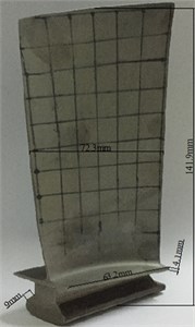
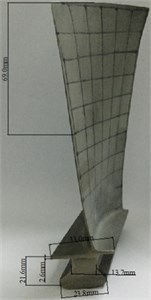
Table 1Typical operational conditions
Case | Take off | Maximum continuous | Cruise | Descending | Flight idle | Ground idle |
Rotational speed / rpm | 9561 | 9337 | 9172 | 8847 | 6966 | 6278 |
3.1.2. Point-cloud data acquisition and digital fitting of blades
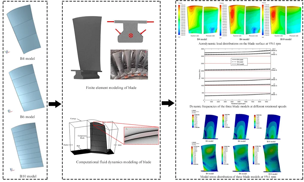
To obtain a computational model that was highly consistent with the real blade and ensure the accuracy of subsequent computations, the blade was digitally scanned using an ATOS mobile high-speed precision optical measurement system (GOM GmbH, Germany). Thereby, a 3D point-cloud model of the compressor blade was obtained (Fig. 2). Fig. 3 shows a flowchart for fitting the point-cloud data. By processing the point-cloud data (including steps such as smoothing, simplifying, extracting, and fitting), a 3D solid model of the blade was established.
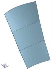
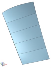
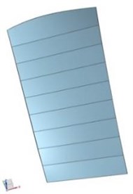
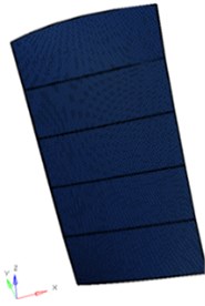
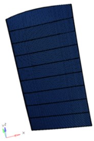
During the reconstruction of the blade surface, a certain number of profile lines were used for boundary control to ensure accurate reverse modeling of the blade surface. However, increasing the number of profile lines increases the complexity of the digital modeling and the work difficulty. To investigate the effect of the means of modeling on the numerical computation, three reverse-modeling solutions were proposed in this study: reconstruction of the blade surface using four, six, or ten curves to fit the blade profile along the span direction (designated as B4, B6, and B10, respectively, as shown in Fig. 4). The blade surface was then reconstructed using the envelopes of the leading and trailing edges and the surface profile curves as constraints and fitting the internal point-cloud data using a least-squares method. In this way, three solid models of the blade were obtained by extending, assembling, and trimming the fitted surfaces (Fig. 5).
Fig. 2Blade geometry data acquisition
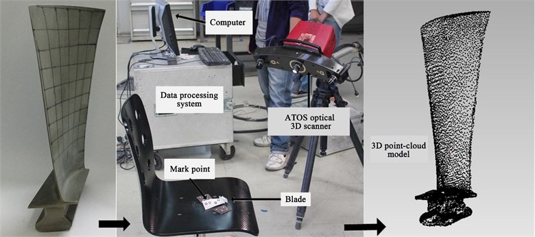
Fig. 3The flow chart of point-cloud data fitting
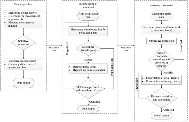
Fig. 4Reverse modelling strategy for the blade
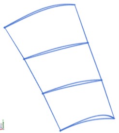
a) Project 1: 4 section profiles
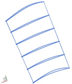
b) Project 2: 6 section profiles
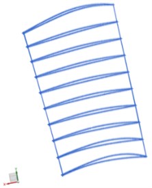
c) Project 3: 10 section profiles
Fig. 5Entire reverse modelling process for the blade
a) B4 model
b) B6 model
c) B10 model
3.2. FE modeling of the blade and model verification
To better reflect the thin-wall characteristics of the blade, the 3D blade models were gridded using ten-node tetrahedron elements (Solid 187). Fig. 6 shows the FE blade models, and Table 2 shows their mesh parameters. To eliminate the effect of the grid number on the computational accuracy, the three models were gridded using numbers of the same order of magnitude. The error between the result obtained using the largest grid number and that using the smallest grid number, , was controlled below 0.02. The value of is computed using:
Fig. 6FE modelling for the blade
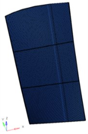
a) B4 model
b) B6 model
c) B10 model
Table 2Grid and node numbers for each blade FE model
Blade model | B4 | B6 | B10 |
Grid number (GN) | 302,048 | 321,470 | 317,218 |
Node number (NN) | 666,983 | 734,995 | 692,527 |
Based on the actual way in which the blade is attached to the disk, constraints were applied to the tenon-and-mortise joint as follows: the tenon-mortise interface was subject to a normal constraint, the front and rear edges of the tenon were subject to an axial constraint, and the T-step was subjected a radial constraint (Fig. 7). The compressor blade was made from a titanium alloy Ti-6Al-4V, whose major mechanical properties are [15]: density 4440 kg/m3; modulus of elasticity 1.07×10⁵ MPa; and Poisson’s ratio 0.3.
Modal computation was performed on the three FE blade models and the results were then compared with the modal test results of the blade to verify the accuracy of the modeling. The model tests were performed using a single-excitation, single-response method (Fig. 8). The test equipment included a PSV-400-3D Scanning Vibrometer system (Polytec, Germany) and a Test.Lab Vibration Control test system (LMS International). The laser probe of the PSV-A-400 (Fig. 9) was used as the acceleration signal sensor in the test. This non-contact measurement device obtains the response of the blade to the excitation by detecting the variation in the displacement of spatial points. The test process is simple and is not affected by the added mass. The excitation forces were measured using a piezoelectric force sensor, and the displacement responses at the measurement points were measured using the non-contact laser optical probe. The collected signals were transferred to signal processing system for computer processing of data analysis.
Fig. 7The constraint conditions of blade FE model
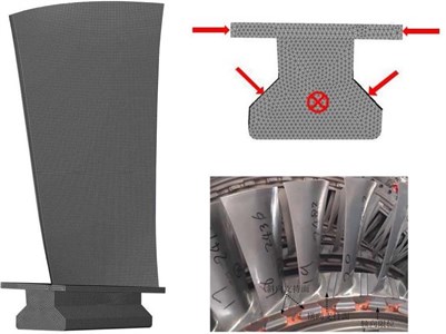
Fig. 8Modal test of the blade
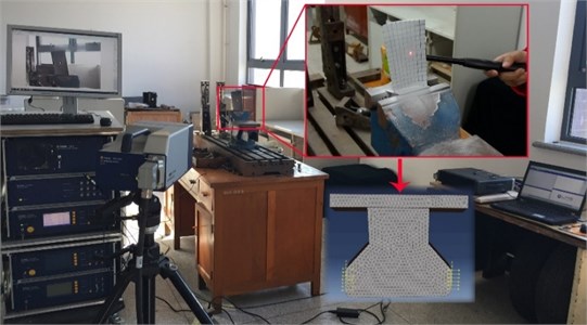
Table 3 shows a comparison of the modal computation results obtained using the three blade models and the experimental results. The errors between the numerical results of the natural frequencies of the first six modes obtained using the FE models of the blade and the experimental results were below 10 %, confirming that the three models satisfied the requirements for subsequent computations. The errors may be caused by the following factors: 1) differences between the computational models of the blade and its actual structure, and 2) differences between the simulated and actual boundary conditions for constraining the blade’s displacement.
Further analysis revealed that the first, second, and fifth-order frequencies of model B4 had large errors when compared with the experimental results. The low-order frequencies of model B10 were relatively accurate. The frequencies of model B6 in the different modes were close to the corresponding values of model B10, and the frequency computation error varied only slightly across the modes. The computational results of mode shape for the three blade models differed only insignificantly from the experimental results. For example, the fifth mode shape of the three models (Fig. 10) exhibited consistently large deformations in the two top corners of the blade tip and the middle regions of the leading and trailing edges. The different modeling approaches meant that the blade models had different natural frequencies and corresponding modes of vibration. These differences in the vibration characteristics of the three blade models are subject to further investigation.
Fig. 9The major equipment of modal test
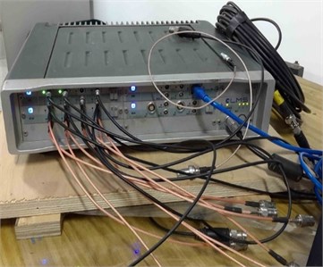
a) Test.Lab Vibration Control test system
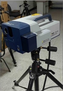
b) Laser probe of the PSV-A-400
Table 3Comparison of computational modal and test modal
Mode No. | Experimental results (Hz) | Computation results of FE (Hz) | Relative error (%) | ||||
B4 | B6 | B10 | B4 | B6 | B10 | ||
1 | 272.94 | 296.07 | 284.90 | 279.97 | 8.47 | 4.38 | 2.58 |
2 | 956.94 | 1016.80 | 1006.80 | 999.41 | 6.27 | 5.21 | 4.44 |
3 | 1283.13 | 1256.30 | 1256.50 | 1244.00 | 2.09 | 2.08 | 3.05 |
4 | 2133.93 | 1961.00 | 1950.60 | 1938.20 | 8.10 | 8.59 | 9.17 |
5 | 2752.60 | 3025.70 | 3011.20 | 3005.30 | 9.92 | 9.39 | 9.18 |
6 | 3238.47 | 3196.50 | 3172.00 | 3168.70 | 1.29 | 2.06 | 2.15 |
Fig. 10Comparison of the fifth mode shape between FE model and experiment
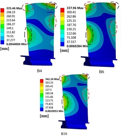
a) Computational results of mode shape
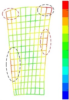
b) Experimental results of mode shape
3.3. Modeling of blade flow field and model validation
During the operation of the engine, the blade is subject to centrifugal load induced by its rotation, the aerodynamic load induced by the airflow, and the resulting vibration load. The blade vibrates under the combined effect of the centrifugal and aerodynamic loads, resulting in a complex stress state and changes in its vibration characteristics. Therefore, to understand the internal flow characteristics of the compressor and determine the aerodynamic loads on the blade surface at different rotational speeds, computational models of the blade flow field were established (Fig. 11). The three blade flow-field models differed mainly in the number of flow-field mesh cells, but all were gridded using multiple-block structured mesh topologies and were configured with the same parametric settings as follows: blade tip gap 1.7 mm; length of inlet flow path 80 mm; length of outlet flow path 120 mm. The pressure distributions on the compressor blade surface under the six typical operating conditions were numerically simulated using the Ansys Fluent 17.0 software package. Considering that the flow field to be computed is in a turbulent flow state, the – turbulence model and the standard wall functions were used, and these were solved using the explicit algorithm and the second-order upwind scheme. The boundary conditions were defined as follows: pressure inlet and outlet; front and rear walls: rotational periodic boundary; bottom wall: no-slip boundary condition. Table 4 shows the number of cells and number of nodes used to grid the three blade flow-field models.
Fig. 11Computational fluid dynamics modeling of blade
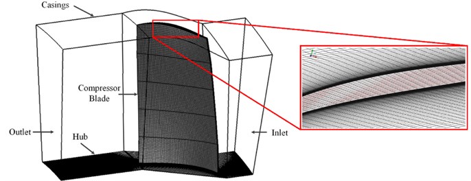
Table 4Element and node numbers for each blade flow-field model
Blade model | B4 | B6 | B10 |
Cell number | 1,394,679 | 1,389,481 | 1,395,352 |
Node number | 1,617,240 | 1,609,863 | 1,615,733 |
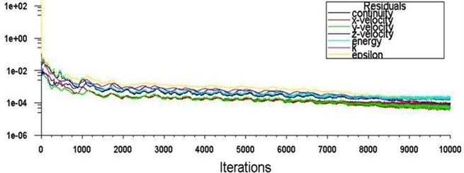
Fig. 12 shows the convergence residuals for iterative calculations of blade model B6 to verify the flow-field model. When the number of iterations rose to 8000, the residuals were less than 10-3, that is to say iterative calculation was tending towards stability.
Fig. 12Residuals of iterative calculations
4. Results and discussion
4.1. Aerodynamic pressure characteristics
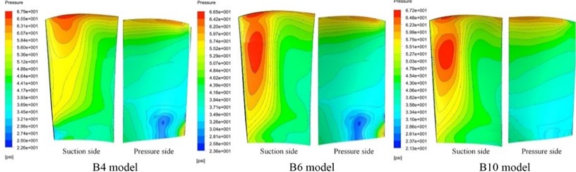
In the compressor structure, the aerodynamic load induced by the interaction between the airflow and blade rotation is the major causal factor of the blade vibration. When the blade vibrates, if the aerodynamic force continuously inputs energy into the blade system, then high vibration pressure will be generated, leading to fatigue fracture of the blade. Fig. 13 shows the aerodynamic load distributions on the blade surface at a rotational speed of 9561 rpm obtained using the three blade flow-field models. The aerodynamic pressure distributions on the pressure side of models B4 and B6 were basically consistent, but the aerodynamic pressure distributions on the suction side differed significantly. In model B4, the maximum aerodynamic pressure zone was mainly located near the blade tip, whereas in model B6, the maximum aerodynamic pressure zone was mainly located at 3/4 blade height. In contrast, the aerodynamic pressure distributions on the suction sides of models B6 and B10 were consistent, whereas those on the pressure side differed to a certain degree.
Fig. 13Comparison of aerodynamic load distributions on the blade surface at 9561 rpm
The aerodynamic pressures on the blade surface at 50 % blade height at 6278 and 9337 rpm were compared. As shown in Fig. 14(a), at low rotational speed, the three blade models had similar surface aerodynamic pressure variations. In particular, the aerodynamic pressure distributions of B6 and B10 were more consistent when compared with those of B4. As shown in Fig. 14(b), at high rotational speed, the surface aerodynamic pressure variations of model B4 were larger than those of the other two models, and that the surface pressure of models B6 and B10 were also approximative. As revealed by the above comparative analysis, the accuracy of blade-profile fitting greatly affects the blade flow-field computation.
Fig. 14Comparison of aerodynamic pressures at 50 % blade height at two rotational speeds
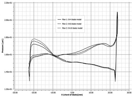
a) 6278 rpm
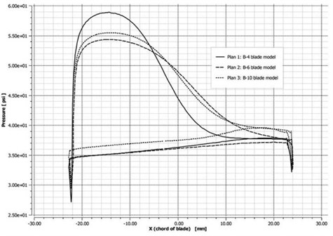
b) 9337 rpm
4.2. Frequency analysis
Each blade is subject to complex centrifugal and aerodynamic loads when rotating with the blade disk. The centrifugal force, which acts in the blade span direction, increases the bending stiffness of the blade, while the aerodynamic load causes torsional deformation. Thus, the blade has different natural frequencies in its rotating and static states. When the external excitation load is consistent with the blade’s natural frequency, the blade produces a resonance state and experiences large vibration stress. Therefore, the dynamic frequencies of the three blade models were calculated to analyze the effect of the surface-fitting parameters of reverse modeling on the blade’s frequency characteristics.
Fig. 15Dynamic frequencies of the three blade models at different rotational speeds
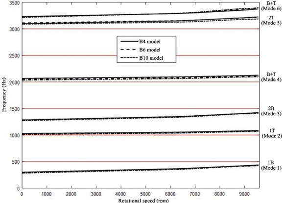
As shown in Fig. 15, the three blade models exhibited similar dynamic frequency variations with the rotational speed. At low speeds, the low-order modal frequencies of the different models varied with the rotational speed in basically consistent patterns. As the rotational speed continued to increase, the high-order modal frequencies varied with larger magnitudes, and the frequencies in the different modes differed significantly. At the maximum rotational speed (9561 rpm), the difference between the fifth-mode frequency of model B4 and that of model B10 was 105.2 Hz, whereas the modal frequencies of models B6 and B10 were relatively consistent (Table 5). Because the blade is twisted, so that the surface precision has effect on the numerical computation. In the high order torsional deformation, the error of different models is larger. Thus, for low-order modes, the number of profile lines used for the reverse modeling of the blade had an insignificant effect on the computation, whereas for high-order modes, an appropriate blade model needs to be selected according to the required computational accuracy.
Table 5Modal frequency and shape of the three blade models at rotational speed 9561 rpm
Mode No. | 1 | 2 | 3 | 4 | 5 | 6 |
Frequency of B4 model (Hz) | 438.12 | 1086.0 | 1419.5 | 2123.2 | 3231.5 | 3357.6 |
Frequency of B6 model (Hz) | 430.04 | 1063.1 | 1429.2 | 2093.6 | 3160.9 | 3386.8 |
Frequency of B10 model (Hz) | 424.95 | 1053.7 | 1412.2 | 2081.8 | 3126.3 | 3381.9 |
Modal shape | 1st order bending (1B) | 1st order torsion (1T) | 2nd order bending (2B) | Bending and torsion (B+T) | 2nd order torsion (2T) | Bending and torsion (B+T) |
Table 6Dynamic frequencies of the B6 model at different rotational speeds under different load conditions
Mode No. | load condition | Dynamic frequency/Hz | |||||
6278 (rpm) | 6966 (rpm) | 8847 (rpm) | 9172 (rpm) | 9337 (rpm) | 9561 (rpm) | ||
1 | CL | 357.78 | 371.62 | 413.15 | 420.77 | 424.68 | 430.04 |
CL+ AL | 356.81 | 370.61 | 412.06 | 419.48 | 423.37 | 428.63 | |
2 | CL | 1040.6 | 1044.9 | 1057.9 | 1060.2 | 1061.4 | 1063.1 |
CL+ AL | 1044.4 | 1050.3 | 1068.6 | 1072.2 | 1074.2 | 1076.2 | |
3 | CL | 1348.7 | 1363.1 | 1409.3 | 1418.2 | 1422.8 | 1429.2 |
CL+ AL | 1347.6 | 1361.3 | 1404.8 | 1413.5 | 1417.9 | 1423.6 | |
4 | CL | 2069.7 | 2073.9 | 2087.5 | 2090.2 | 2091.6 | 2093.6 |
CL+ AL | 2078.8 | 2084.6 | 2103.8 | 2107.9 | 2109.9 | 2112.5 | |
5 | CL | 3136.3 | 3140.8 | 3154.8 | 3157.5 | 3159.0 | 3160.9 |
CL+ AL | 3153.5 | 3164.6 | 3200.3 | 3207.9 | 3211.7 | 3216.0 | |
6 | CL | 3288.7 | 3305.8 | 3362.0 | 3373.1 | 3378.8 | 3386.8 |
CL+ AL | 3290.9 | 3307.7 | 3365.1 | 3378.2 | 3384.5 | 3391.9 | |
Note: CL denote only centrifugal load, and CL+ AL denote both centrifugal and aerodynamic loads | |||||||
In addition, as revealed by the above analysis of the aerodynamic pressure on the blade surface, the coupling effect of the airflow excitation and the centrifugal load affects the blade’s dynamic frequency characteristics. Therefore, the dynamic frequencies of model B6 at typical rotational speeds under different loading conditions (Table 6) were analyzed to investigate the effect of the loading parameters on the blade’s frequency characteristics.
The natural frequencies of the blade in the different modes increased with the rotational speed (Table 6). This is because the load on the blade resulting from the rotation increases the blade’s stiffness, thereby increasing the frequency. In particular, the sixth-mode frequency increased by the largest magnitude, whereas the first-mode frequency increased by the largest ratio due to its relatively low frequency. This is because the natural frequency of a structure is in direct proportion to its stiffness; however, the natural frequency does not increase infinitely as the stiffness increases, i.e., increasing the stiffness can only increase the natural frequency by a certain magnitude.
With the airflow excitation considered, the blade’s modes of vibration at different orders did not vary as the engine’s rotational speed varied; however, the magnitude of the dynamic frequency did vary. With the effect of the aerodynamic pressure considered, the blade’s first- and third-order frequencies decreased slightly, whereas the second-, fourth-, fifth-, and sixth-order frequencies increased; that is to say, when the airflow excitation is considered, the frequencies in modes dominated by bending deformation decreased, whereas those dominated by torsional deformation increased. The reason behind this phenomenon is as follows. During the operation of the compressor, the tensile–compressive stress caused by the centrifugal load increases the bending deformation of the blade, whereas the aerodynamic load weakens the bending of the blade. In addition, because of the initial twist angle of the blade, considering the airflow excitation further increases the torsion effect of the blade. Therefore, compared with the blade’s dynamic frequency considering the centrifugal load alone, the models also considering the airflow excitation had lower bending frequency but higher torsional frequency, and they better approximated the blade under the real-world operating conditions of the engine.
4.3. Analysis of modal stress
As revealed by the results of modal analysis, the three models differed significantly in their high-order modal frequencies. Therefore, the fifth-order modal stresses of the three models considering the coupling effect of the centrifugal and aerodynamic loads were analyzed to investigate the variations in the modal stress distributions and magnitudes for the different models.
Fig. 161st modal stress distribution of three blade models at 9561 rpm
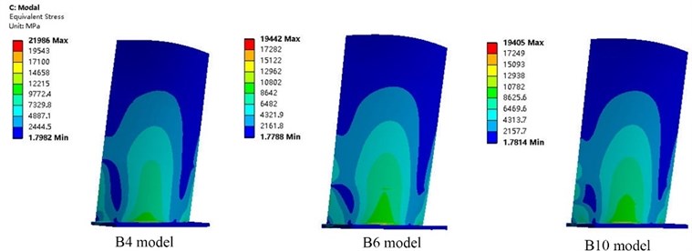
Fig. 175th modal stress distribution of three blade models at 9561 rpm
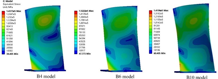
Fig. 16 and Fig. 17 show the first-order modal and fifth-order modal stress distributions of models B4, B6, and B10 at a rotational speed of 9561 rpm. The first-order mode was first-order bending, and the stress distributions were similar. However, the fifth-order modes of vibration of the three models were consistently second-order torsion, and the models differed in the location of maximum stress and stress concentration: for model B10, the fifth-mode maximum stress was located at a position on the rear edge of the blade at 15 mm from the blade root, whereas for models B4 and B6, the fifth-mode maximum stress was located near the blade root in an area of stress concentration. Because the fifth-order mode of vibration of the blade was second-order torsion and the compressor blade is a variable-chord (thin front and rear edges), twisted blade, the blade experienced large vibration displacement at the blade root on the rear edge, resulting in a large stress concentration in this region. Stress concentration also occurred in the location with a symmetric cross-section of second-order torsional deformation. Long-term blade service data have shown that fatigue cracks initiate in blades in areas of stress concentration. Therefore, the cause of blade resonance failure can be preliminarily determined based on blade modal stress analysis.
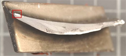
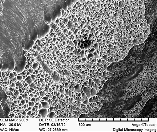
An analysis of the characteristics of the historical faults of this blade revealed that damage occurred at the front and rear edges near the blade root (Fig. 18). As revealed by the above numerical computation results, the location of the concentration of modal stress in the blade (Fig. 17) roughly coincides with the blade fatigue crack initiation zones (Fig. 18). The morphology of the fatigue fracture surface was further analyzed, and the crack initiation areas and the fatigue propagation areas are indicated in the Fig. 18. The fracture surface was bright and coarse. This indicates that, when resonance occurs, the blade experiences high stress and rapid fatigue propagation at the blade root, finally leading to fatigue failure.
Fig. 18The fatigue fracture surface features of blade
5. Conclusions
In this study, 3D models of a compressor blade for an aero engine with three different levels of surface accuracy (designated B4, B6, and B10) were established via digital fitting engineering by the blade profile coordinates. Then, the numerical models including finite element and flow-field models of the blade were established and validated. Considering both the aerodynamic excitation and the centrifugal load, the vibration characteristics of the blade were analyzed under different operating conditions. The main conclusions are as follow:
1) The errors of modal frequency between calculation and experiment for the three blade models were all less than 10 %. Although the frequency values of three blade models were different, the modal shape of those models were consistent with the experiment. Thereby, the numerical models (designated B4, B6, and B10) all met the demand of engineering computation.
2) Under complex centrifugal and aerodynamic loads, the three blade models differed significantly in their high-order dynamic frequencies, since the bending and torsion characteristics of those models are different. The modal frequencies that were dominated by a torsional mode of vibration were sensitive to the aerodynamic load and the modal frequencies dominated by a bending mode of vibration were sensitive to the centrifugal load. Thereby, considering both the aerodynamic and the centrifugal load increased the accuracy of the numerical computation of the blade vibration characteristics.
3) Comparing the computational results of three blade models, it is found that, models B6 and B10 differed only insignificantly, and B6 decreased the complexity of the modeling process while satisfying the required computational accuracy. To analyze the vibration characteristics of serving blade, accuracy of surfaces fitting for twisted compressor blade is an important indicator to measure the quality of numerical calculation.
References
-
W. N. Huang and Z. X. Li, Foreign Aero-Engine Corcise Handbook. (in Chinese), Northwestern Polytechnic University Press, 2014.
-
K. Siddappaji, M. G. Turner, and A. Merchant, “General capability of parametric 3D blade design tool for turbomachinery,” in ASME Turbo Expo 2012: Turbine Technical Conference and Exposition, pp. 2331–2344, Jun. 2012, https://doi.org/10.1115/gt2012-69756
-
Ahmed Nemnem, “An automated 3 D turbomachinery design and optimization system,” Journal of Multidisciplinary Engineering Science and Technology, Vol. 2, No. 11, pp. 3345–3359, Jan. 2015.
-
R. A. Alexeev, V. A. Tishchenko, V. G. Gribin, and I. Y. Gavrilov, “Turbine blade profile design method based on Bezier curves,” in Journal of Physics: Conference Series, Vol. 891, No. 1, p. 012254, Nov. 2017, https://doi.org/10.1088/1742-6596/891/1/012254
-
A. W. Leissa, J. K. Lee, and A. J. Wang, “Rotating blade vibration analysis using shells,” Journal of Engineering for Power, Vol. 104, No. 2, pp. 296–302, Apr. 1982, https://doi.org/10.1115/1.3227279
-
M. Berthillier, C. Dupont, R. Mondal, and J. J. Barrau, “Blades forced response analysis with friction dampers,” Journal of Vibration and Acoustics, Vol. 120, No. 2, pp. 468–474, Apr. 1998, https://doi.org/10.1115/1.2893853
-
E. Poursaeidi, A. Babaei, M. R. Mohammadi Arhani, and M. Arablu, “Effects of natural frequencies on the failure of R1 compressor blades,” Engineering Failure Analysis, Vol. 25, pp. 304–315, Oct. 2012, https://doi.org/10.1016/j.engfailanal.2012.05.013
-
K. Kim and Y. S. Lee, “Modal characteristics and fatigue strength of compressor blades,” Journal of Mechanical Science and Technology, Vol. 28, No. 4, pp. 1421–1429, Apr. 2014, https://doi.org/10.1007/s12206-014-0129-z
-
W. Wei et al., “Forced response of aeroengine centrifugal compressor due to impeller-diffuser interaction,” (in Chinese), Structure and Environment Engineering, Vol. 47, No. 3, pp. 24–30, 2020.
-
L. Witek, “Numerical stress and crack initiation analysis of the compressor blades after foreign object damage subjected to high-cycle fatigue,” Engineering Failure Analysis, Vol. 18, No. 8, pp. 2111–2125, Dec. 2011, https://doi.org/10.1016/j.engfailanal.2011.07.002
-
L. Zhang et al., “Vibration analysis of the compressor blade in a gas turbine,” (in Chinese), Journal of Engineering for Thermal Energy and Power, Vol. 34, No. 1, pp. 34–39, 2019.
-
J. D. Brandsen, “Prediction of axial compressor blade vibration by modelling fluid-structure interaction,” Stellenbosch University, Stellenbosch, 2013.
-
P. Dhopade, A. J. Neely, J. Young, and K. Shankar, “High-cycle fatigue of fan blades accounting for fluid-structure interaction,” in ASME Turbo Expo 2012: Turbine Technical Conference and Exposition, pp. 1365–1372, Jun. 2012, https://doi.org/10.1115/gt2012-68102
-
A. Delgado-Gutiérrez, D. Cárdenas, and O. Probst, “An efficient and automated method to generate complex blade geometries for numerical analysis,” Advances in Engineering Software, Vol. 127, No. 1, pp. 38–50, Jan. 2019, https://doi.org/10.1016/j.advengsoft.2018.09.007
-
X. Fu, J. Zhang, and J. Lin, “Study on the fatigue life and damage accumulation of a compressor blade based on a modified nonlinear damage model,” Fatigue and Fracture of Engineering Materials and Structures, Vol. 41, No. 5, pp. 1077–1088, May 2018, https://doi.org/10.1111/ffe.12753
Cited by
About this article

The authors wish to acknowledge the financial support from the Chinese National Natural Science Foundation under Grant No. 51905382.
