Application of PCA-K-means++ combination model to construction of light vehicle driving conditions in intelligent traffic

The construction of typical driving condition of vehicles in line with the actual road traffic conditions in China requires the selection of the same vehicle for two months to collect driving data and the obtention of 496000 driving condition data of light vehicles. The sample data are preprocessed by using multivariate statistical theory and MATLAB. After the elimination of abnormal data, the effective data are extracted before being divided into 3020 kinematic segments. Then, it takes a principal component analysis to reduce the dimension of the characteristic parameter matrix. Through K-means++ clustering algorithm, the six principal components obtained by principal component analysis are clustered into two categories. Then the typical kinematic segments are selected from various fragment libraries by using correlation coefficient method, so as to construct a typical driving condition of the vehicles in a certain city. With the application of PCA-K-means and PCA-K-means++ clustering algorithm, a driving condition curve with a duration of 1200s is constructed before its effectiveness and accuracy being compared and analyzed. The results show that the error rate of driving condition between sample data and driving condition constructed by PCA-K-mean++ clustering algorithm is less than 6 % and the error rate of average speed and acceleration standard deviation is less than 1 %. The correlation degree between working condition curve constructed by PCA-K-means ++ clustering algorithm and sample data is increased by 4.08 %. The proportion of deceleration time and idle time in vehicle driving state is obviously different, which indicates that PCA-K-means++ is a better way to solve the problem and the clustering algorithm can effectively construct the driving condition curve of light vehicles suitable for local cities.

Application of PCA-K-means++ combination model to construction of light vehicle driving conditions in intelligent traffic

1. Introduction

Vehicle driving condition is the main calibration for optimization of vehicle performance indicators, which can be used to evaluate vehicle exhaust emissions, fuel consumption and other indicators. Since this century, China has mainly used NEDC driving condition of Europe and world light test cycle (WLTC) working conditions as references to optimize vehicle performance and carry out calibration, so as to give authoritative results on vehicle economy and emission.

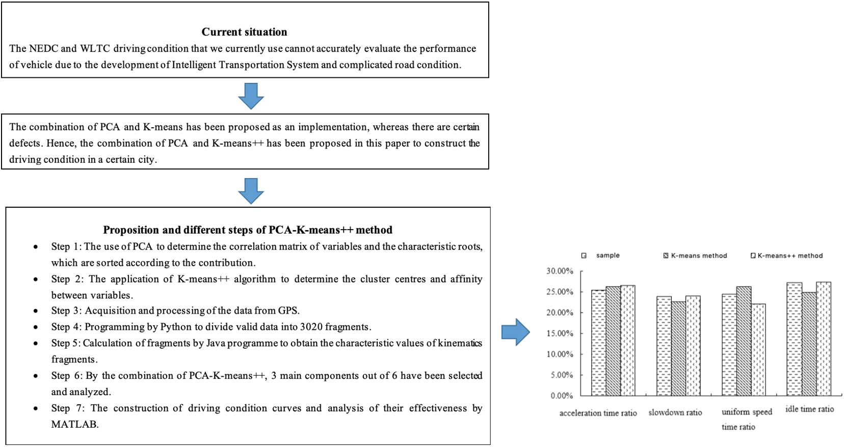
With the acceleration of urban construction, the urban road network is becoming increasingly complex and the traffic flow situation has changed greatly. The two driving condition standards of NEDC and WLTC can no longer be adapted to the traffic situation under the background of intelligent transportation. According to statistics, the error between the driving condition of vehicles based on NEDC and WLTC and the actual operating conditions of automobiles in China is as high as 35 %. Therefore, in a certain area, the construction of accurate vehicle driving condition can provide reference for the test of vehicle emission and fuel consumption, as well as the technical development and evaluation of new models.

At present, researchers all over the world have carried out in-depth study on the driving condition of vehicles, fitted the driving condition of vehicles in line with the traffic characteristics of various regions. In the process of constructing the vehicle driving condition, most researchers combine principal component analysis (PCA) with K-means clustering algorithm in the construction of vehicle driving condition, which brought the following results. Cai [1] et al. applied K-means clustering method to construct the driving condition of Xi’an City, whereas an optimization of the clustering centre has not been carried out. Hence, its application has limitations to some extent. Qin [2] et al. used K-means clustering algorithm to construct driving conditions, which did not optimize the initial value and affected the accuracy. Shi [3] et al. improved the selection of initial value in K-means clustering method by using neural network method, but the clustering quality was reduced due to the lack of clear definition of parameter value K. Gao [4] et al. used the global K-means clustering algorithm to construct the driving conditions to optimize the cluster centre, which improved the robustness of traditional K-means clustering. However, the classification results of the K-means algorithm still depend on the selection of the initial point. Therefore, on the basis of K-means, this paper uses K-means ++ clustering algorithm to construct vehicle driving condition, analyses the accuracy and effectiveness of vehicle driving condition, and finally constructs the driving condition of light vehicle in a city of China.

Through the investigation of vehicles and road conditions in a city, it is found that the car ownership is more than 2.7 million, while the construction of passenger car driving condition is less. Therefore, this paper uses the real-time vehicle driving condition data collected in a city as the sample, using MATLAB to pre-process the original data, dividing the kinematic segments and K-means++ clustering, and in the end obtaining the best among all kinds of cluster centres. At the same time, the abnormal data are processed to extract the kinematic segments, which accord with the actual motion characteristics of the vehicle. Then, the dimension of the collected data is reduced based on kinematic fragment analysis and principal component analysis, 3020 segments are calculated with Java language, the corresponding kinematic segment eigenvalues are obtained, the driving condition of a city road is constructed. Finally, the accuracy of the driving condition is verified by comparing with k-means algorithm and the total sample data collected.

2. Model approach

2.1. Kinematic fragment

The process of frequent starting, accelerating and decelerating is actually a kinematic process. This process is affected by traffic conditions or traffic flow. Therefore, there will be continuous starting and stopping operations during the process from starting to stopping, so it can be regarded as composed of multiple “stop drive stop” segments. In order to simulate the frequent starting, accelerating, decelerating and other driving states of the vehicle in the actual driving process, the driving process from one idle state to the next is defined as a kinematic segment, which is usually composed of an idle part and a moving part [5], as shown in Fig. 1.

Fig. 1Schematic diagram of kinematics

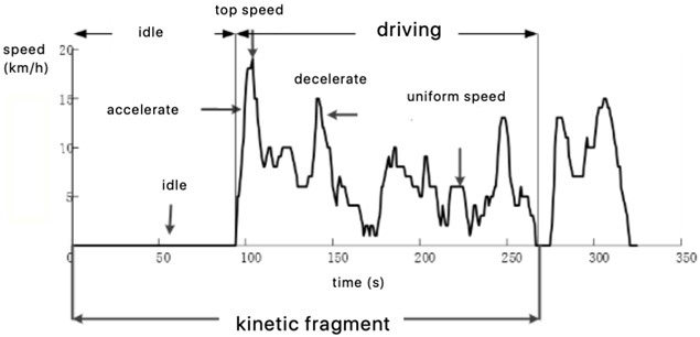
In order to fully express the characteristics of each kinematic segment, according to research [6, 7], the division criteria of four operating conditions are defined in this article.

1) Idle speed: speed $V =$ 0, the engine is idling.

2) Acceleration: Driving state with speed $V \neq$ 0 and $a \geq$ 0.1 m/s².

3) Deceleration: Driving state with speed $V \neq$ 0 and $a \leq$ –0.1 m/s².

4) Constant speed: Driving state with speed $V \neq$ 0 and $|a| \leq$ 0.1 m/s².

Among them, v represents the speed, a represents the acceleration.

2.2. Principal component analysis

Principal component analysis (PCA) is a statistical method to reduce the dimension of high-dimensional data. According to the projection principle, the high-dimensional data is projected on the low-dimensional space with the minimum possibility, which can greatly simplify the data structure. At the same time, it is also a method to combine multiple related variables into a few unrelated variables based on the principle of minimizing data loss. Specific steps are shown in Fig. 2.

Fig. 2Calculation steps of principal component analysis

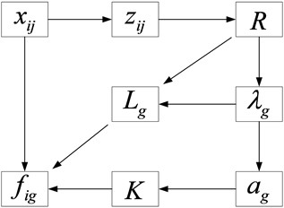
The calculation process is as follows:

Step 1: standardization of index parameters

Since the dimension of each parameter is different, the value of variables is dispersed greatly and the changing range of data affects the clustering effect. Therefore, it is necessary to standardize and dimensionless process each parameter. The Z-score method, which is a non-dimensional method, is used to normalize the parameters of the raw matrix before obtaining the Eq. (1):

1

z_{i j} = \frac{x_{i j} - {\bar{x}}_{i j}}{s_{j}},

where $\bar{X_{j}}$ is the mean value of the $j$ th object and $S_{i j}$ is the standard deviation of the $j$ th object.

Step 2: Determination of the correlation coefficient matrix $R$ between parameters:

2

R = {|r_{j k}|}_{m \times m}, r_{i j} = 1,

3

r_{j k} = r_{k j},

4

r_{j k} = \frac{1}{n - 1} \sum_{i = 1}^{m} z_{i j} z_{i k} .

Step 3: Determination of the characteristic roots of $R$ under the form of $λ_{g} = (1,2, \dots, m)$ , which describes the importance of each component:

5

|λ_{g} I_{m} - R| = 0 .

Step 4: Determination of the eigenvectors of the $R$ matrix, where $L$ is an m-dimensional vector:

6

|λ_{g} I_{m} - R| L_{g} = 0 .

Step 5: Determination of the contribution rate of the $R$ -array:

7

a_{k} = \frac{λ_{g}}{\sum_{g = 1}^{m} λ_{g}} .

Step 6: Determination of the number $K$ of principal components. Sort the components according to the contribution rate. If the original number is large, the first $K$ are taken to represent all the quantities:

8

a (K) = (\sum_{g = 1}^{K} λ_{g}) {(\sum_{g = 1}^{m} λ_{g})}^{- 1} .

According to determining the number of principal components, $m$ related indicators can be reduced to $K$ unrelated principal components:

9

f_{i k} = \sum_{j - 1}^{m} L_{i j} z_{i j} .

2.3. K-means++ clustering method

2.3.1. K-means++ algorithm theory

Aiming at big data clustering, K-means++ algorithm is the optimization of random initialization centroid method of K-means. Comparing with other K-means clustering algorithms, the advantage of K-means++ clustering algorithm is that it takes the farthest possible distance as the data selection principle as the initial clustering centre. Besides, the selected initial cluster centre can be optimised. Therefore, the algorithm solves the problem of initial value selection, improves the stability of the algorithm and the robustness of clustering results that rely too much on the initial cluster centre.

The method of K-means++ clustering algorithm to select the initial center point is: first, considering the distribution of all samples in the data set, the distance between the selected initial center points should be as far as possible, so as to avoid the problem of large clusters being divided or several smaller clusters being wrongly merged.

Assuming that $D = \{X_{i} |X_{i} \in R^{m}, i = 1,2, \dots, n\}$ represents the data set of the sample, $m$ represents the data dimension and n is the set size. Assuming that $C = {C_{k} |C_{k} \in R^{m}, i = 1,2, \dots, k}$ represents the class to which the sample set belongs, then $k$ represents the number of category belonged, $C^{0}$ represents the initial clustering centre, the formula for calculating the distance between samples is as following:

10

D i s t (X_{i}, Y_{j}) = \sqrt{{(X_{i} - Y_{j})}^{T} (X_{i} - Y_{j})} .

Cluster centre:

11

c_{k} = \frac{1}{n_{k}} \sum_{x_{i} \in c_{k}} X_{i} .

The basic theory of K-means++ clustering [8] is that based on the set $K$ value and algorithm, samples are continuously selected from the class whose cluster centre is randomly chosen. When $E$ is the smallest (setting function is optimal), the process terminates. The result of the algorithm is to divide a large number of samples into different classes, showing different population aggregation distributions. The characteristic is that the distance is small between the internal sample elements of the class, while the distance is large between the classes:

12

E = \sum_{i = 1}^{k} \sum_{j = 1}^{n} D i s t (X_{j}, c_{i}) .

The workflow of K-means++ algorithm is as follows:

1) A sample in dataset $D$ is randomly selected as the first initial cluster centre;

2) The shortest distance between each sample and the current cluster centre is calculated, which is represented by $D (x)$ ;

3) The probability that each sample is selected as the next cluster centre is calculated;

4) According to the principle that probability is proportional to $D (x)$ , a new sample is selected as the cluster centre;

5) When the number of initial cluster centers $K$ is selected, the iteration process is terminated;

6) Re implement the traditional K-means algorithm.

2.4. Correlation analysis

Correlation analysis is an analysis of two or more related variables to describe the closeness between the variables. Correlation coefficient is a statistical analysis index for analysing the correlation degree of straight lines, and the value range is between –1 and 1. –1 indicates that the variables are completely uncorrelated, 0 indicates that they are not related and 1 indicates that they are completely related. The closer the data tends to 0, the weaker the correlation is. The specific calculation formula is shown in Eq. (13):

13

D i s t ρ_{x y} = \frac{C o v (X, Y)}{\sqrt{D (X)} \sqrt{D (Y)}} .

Among them, $C o v (X, Y)$ is the covariance of variables $X$ and $Y$ , $D (X)$ and $D (Y)$ are variances of variables $X$ and $Y$ , respectively. When $ρ_{x y} \geq 0.9$ , high correlation is generally believed between two groups of variables.

3. Data acquisition and processing

3.1. Data collection

The commonly used vehicle data acquisition methods include vehicle tracking method, average vehicle flow statistics method, autonomous driving method, etc. Among them, the autonomous driving method does not need to plan the specific test driving route in advance. Instead, the owner can drive autonomously according to the normal driving habits. In order to make the collected data more effective and fully express the traffic characteristics of a certain sound City, the selected vehicle should consider the location of the owner and the road condition of the owner every day. Therefore, the daily driving route of the selected vehicle should include places with frequent traffic interaction, such as residential areas, schools, stations, parks, etc.

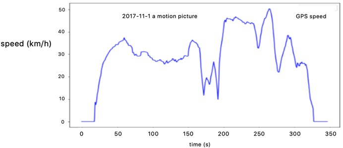
In this paper, the autonomous driving method is used to collect the driving track data of different driving areas and driving periods and the vehicle terminal (GPS) is used to collect the driving data. The data acquisition frequency is set at 1Hz and the real-time vehicle driving data is recorded for about two months from November 1, 2017 to December 24, 2017, including vehicle position (longitude and latitude), speed, time, vehicle fuel consumption, etc. Finally, 496014 driving data were obtained.

3.2. Data pre-processing

In the construction process of vehicle driving condition, the quality of collected data will inevitably decline due to various reasons such as unstable transmission signal, electromagnetic interference, decoding error and so on. In order to improve the data quality and ensure the credibility of the research results, this paper uses MATLAB software to preprocess the original data.

In order to convert a given date string (date) into a date number (time), the datenum function in MATLAB software is used to process the time item according to the following format: Time=datenum(date,'yyyy/mm/dd HH:SS.000').

Since there are some errors in the original data collected directly, this paper analyzes and summarizes the error data according to the structure types, processes them in batches. For the discrete data, linear interpolation is carried out for the abnormal data before the abnormal data being eliminated.

3.2.1. Intermittent data processing

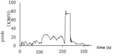
Discontinuities will occur in the data due to interference from weather changes, obstructions, poor signal reception, etc. The data in this case is defined as discontinuous data. The solution for this problem is demonstrated as follows. Clips are deleted that time intervals are greater than 10 s; For data with a time interval less than 10 s, linear interpolation is used to supplement the points. Before and after the discontinuous data is eliminated, the variance of the velocity is shown in Fig. 3 (a) and (b), respectively.

Fig. 3Intermittent data processing

a) Before processing

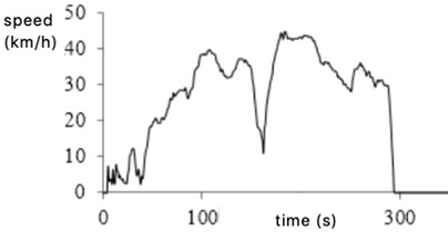
b) After processing

3.2.2. Acceleration and deceleration abnormal data processing

Due to the limitation of the road environment, the accuracy of GPS collected data will be affected, resulting in some abnormal signals. The abnormal data of car acceleration and deceleration is one of them. The acceleration time from 0 to 100 km/h is more than 7 seconds for an ordinary car, and the maximum deceleration is between 7.5-8 m/s² when emergency brakes. According to related bibliography [9], it is defined as abnormal data for the tested vehicle when the acceleration exceeds 3.97 m/s² or the deceleration exceeds 8 m/s², then such data will be deleted. Acceleration and deceleration abnormal data before and after removal are shown in Fig. 4(a) and (b), respectively.

Fig. 4Acceleration and deceleration abnormal data processing

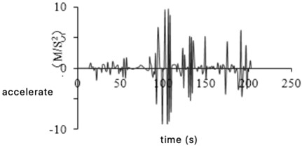
a) Before elimination

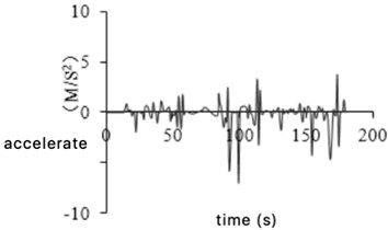
b) After removal

3.2.3. Idle abnormal data processing

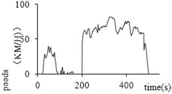
Idle is a continuous process in which the car stops moving but the engine is running at the lowest speed. When the vehicle stopped for a long time, abnormal idling data will appear in the collected valid data due to equipment accuracy. One is the case of stopping and not turning off, that is, the clip with zero speed is less than 20 s; the other is that the car is stopped and the device is to continue running. It is also in a state of zero speed. For this data, a rule aiming for idling abnormal data is formulated, which is filtered and eliminated according to the rules. Fig. 5(a) and 5(b) show the variation of speed before and after the idling abnormal data being eliminated.

Fig. 5Idle abnormal data processing

a) Before processing

b) After processing

3.2.4. Glitch data processing

During the driving process, the idling data collected has abnormal with non-zero speed due to factors such as poor signal. This data is defined as glitch data. This situation does not exist during the actual driving of the car. This paper uses such data, whose continuous driving time is no more than 3 seconds, at the same time its speed is less than 10 km/h, as glitch data. Reference [10] modified this data to zero to identify it as the idling point. Fig. 6(a) and (b) show the glitch data before and after removal.

Fig. 6Glitch data processing

a) Before processing

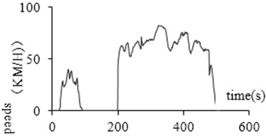
b) After processing

3.2.5. Long idle time abnormal data

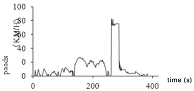
The abnormal idling time refers to the data in which the segment of the holding speed is more than 180 seconds when the vehicle is stationary and the engine continues to work. If the idle is not in this range, one possibility is that the device is abnormal, and the car is not powered off after the car stops, and the device continues to collect information; another is that the car has been left in the same location for a long time without driving. These inconsistent data should be eliminated to reduce the error rate of the construction of the vehicle operating conditions. Fig. 7(a) and (b) before and after removal of the abnormal idling time abnormal data, respectively.

Valid 457550 driving data was obtained after discontinuous data being interpolated, acceleration and deceleration abnormal data being eliminated and idling being deleted, glitch being modified, and long idling time being proceeded.

Fig. 7Abnormal data processing at idle time

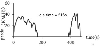
a) Before processing

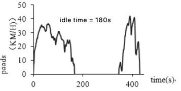
b) After processing

4. Construction of driving condition model and result analysis

On the basis of data preprocessing, the driving condition data can be divided into kinematic segments and different number of characteristic parameters can be selected as principal component analysis.

4.1. Kinematic segmentation

According to the definition of kinematic fragments, the first data is divided into multiple motion segments. Then fragments are select based on valid segment filtering rules. Python programming is used to divide the micro-stroke due to the large amount of experimental data. Since the frequency is 1 Hz, when the fragments are performed, each line of data is reduced to one line, which includes the vehicle speed only [11, 12]. A total of 3020 kinematic segments are obtained by dividing the pre-processed data into kinematic segments. The vehicle operating conditions will be built based on this. The schematic diagram of kinematics is shown in Fig. 8.

Fig. 8Schematic diagram of kinematics

4.2. Construction of driving conditions model

This paper defines 16 feature parameters to describe the operating conditions of all kinematic segments, and 22 to describe the overall distribution characteristics of kinematic segments according to the importance of feature parameters to vehicle driving information. See Table 1 and Table 2 for information on each characteristic parameter. By combining the calculated feature parameter values of all the motion segments, a sample of each segment can be obtained before establishing a matrix of sample numbers (rows) × feature parameters (columns), which is used for the construction of driving conditions.

Table 1Kinematics segment running characteristic parameter information table

Number	Characteristic parameters	Unit	Number	Characteristic parameters	Unit
1	Acceleration time $T_{a}$	%	9	Maximum speed $V_{m a x}$	km/h
2	Deceleration time $T_{d}$	%	10	Minimum speed $V_{m i n}$	km/h
3	Uniform time $T_{c}$	%	11	Acceleration $A_{m a x}$	m/s²
4	Idle time $T_{i}$	%	12	Deceleration $D_{m a x}$	m/s²
5	Operation hours $T_{r}$	S	13	Standard deviation of speed $V_{s}$	km/h
6	Cumulative driving distance $S$	km	14	Standard deviation of acceleration $A_{s}$	m/s²
7	Average speed $V_{m}$	km/h	15	Average acceleration $A_{m}$	m/s²
8	Average running speed $V_{m r}$	km/h	16	Average deceleration $D_{m}$	m/s²

Table 2Feature parameter information table of the overall distribution of kinematics

Number	Characteristic parameters	unit	number	Characteristic Parameters	Unit
1	Acceleration time ratio $P_{a}$	%	12	Speed ratio of 70-80 km/h $P_{70 - 80}$	%
2	Slowdown ratio $P_{d}$	%	13	Ratio of speed greater than 80 km/h $P_{80}$	%
4	Idle time ratio $P_{i}$	%	15	–2 m/s²- –1.5 m/s² acceleration ratio $A_{- 2 ~ - 1.5}$	%
5	Speed ratio between 0~ 0 km/h $P_{0 - 10}$	%	16	–1.5 m/s²- –1 m/s² acceleration ratio $A_{- 1.5 ~ - 1}$	%
6	Speed ratio of 10-20 km/h $P_{10 - 20}$	%	17	– l m/s²- –0.5 m/s² acceleration ratio $A_{- 1 ~ - 0.5}$	%
7	Speed ratio of 20-30 km/h $P_{20 - 30}$	%	18	– 0.5 m/s²-0.5 m/s² acceleration ratio $A_{- 0.5 ~ 0.5}$	%
8	Speed ratio of 30-40 km/h $P_{30 - 40}$	%	19	0.5 m/s²-1 m/s² acceleration ratio $A_{0.5 ~ 1}$	%
9	Speed ratio of 40-50 km/h $P_{40 - 50}$	%	20	1m/s²-1.5 m/s² acceleration ratio $A_{1 ~ 1.5}$	%
10	Speed ratio of 50-60 km/h $P_{50 - 60}$	%	21	1.5 m/s²-2 m/s² acceleration ratio $A_{1.5 ~ 2}$	%
11	Speed ratio of 60-70 km/h $P_{60 - 70}$	%	22	Ratio of acceleration section above 2 m/s² $A_{2}$	%

A program based on the Java language is written to serve for the calculation 3020 fragments and obtain the corresponding running feature values of the kinematic fragments. The characteristic values of all fragments are shown in Table 3.

4.2.1. PCA analysis results

According to the steps of principal component analysis, the eigenvalue matrix is analysed, and six principal components are obtained, which are labelled as $M_{1}$ , $M_{2}$ , $M_{3}$ , $M_{4}$ , $M_{5}$ , $M_{6}$ , and the contribution rate and cumulative contribution rate are calculated, the results are shown in Table 4.

Table 3Kinematic segment feature parameter values

Fragment number	$T_{d}$	$T_{c}$	$V_{m}$	...	$V_{s}$
1	24	76	65.31	...	17
2	39	45	51.11	...	16.78
3	40	29	53.29	...	23.44
4	12	33	34.22	...	0.64
5	26	24	65.8	...	0.53
6	17	31	115.31	...	0.66
7	25	19	87.94	...	19.84
8	33	17	57.4	...	17.78
9	41	60	107.31	...	23.61
...	...	...	...	...	…
3019	9	22	69.66	...	24.21
3020	36	34	78.17	...	0.78

Table 4Analysis results of the main components

Main ingredient	Eigenvalues	Contribution rate (%)	Cumulative contribution rate (%)
$M_{1}$	5.6174	45.8563	95.6584
$M_{2}$	3.1933	19.2535	92.2542
$M_{3}$	1.7534	16.2543	85.5463
$M_{4}$	0.8524	7.2514	63.2015
$M_{5}$	0.2563	3.2541	45.8563
$M_{6}$	0.0452	1.2542	39.7815

By solving the characteristic equation $|λ_{g} I_{m} - R| = 0$ , m nonnegative eigenvalues of the correlation coefficient matrix $R$ can be obtained and arranged in order of magnitude. The larger the eigenvalue of the correlation coefficient matrix is, the better the initial variable can be represented by the representative principal component to a greater extent. The contribution rate represents the degree of reflection on it. Generally, when the cumulative contribution rate reaches 85 %, the information of the initial variable can be reflected. It is concluded from Table 4 that the contribution rate of $M_{1}$ , $M_{2}$ , and $M_{3}$ reaches 85 %, which can represent the information of the initial variables, and their eigenvalues are greater than 1, so the initial characteristic parameters can be characterized by $M_{1}$ , $M_{2}$ , and $M_{3}$ .

Table 5Calculation results of the principal component factor load matrix

Characteristic parameters	$M_{1}$	$M_{2}$	$M_{3}$
$T$	0.559	0.299	0.101
$S$	–0.022	0.846	–0.136
$T_{i}$	0.697	–0.194	0.376
$T_{a}$	0.043	0.714	–0.083
$T_{d}$	0.091	0.615	–0.384
$T_{e}$	0.116	0.263	–0.217
$V_{m a x}$	–0.225	0.947	0.083
$V_{m}$	–0.442	0.866	–0.101
$V_{m r}$	–0.135	0.918	0.018
$V_{s}$	–0.316	0.941	0.290
$A_{m a x}$	0.643	0.535	–0.595
$A_{m}$	0.478	0.464	–0.430
$D_{m a x}$	0.064	0.689	0.533
$D_{m}$	0.064	0.680	0.532
$A_{s}$	0.386	0.544	–0.038

According to the contribution table of the principal components, we choose to end the accumulation when the cumulative contribution rate exceeds 80 %. The factor load matrix is calculated by the characteristics of the first three components whose cumulative contribution rate is greater than 85 %. The calculation results are shown in Table 5.

As can be seen from Table 5, $M_{1}$ mainly reflects the idle time; $M_{2}$ mainly reflects the running distance, acceleration time, deceleration time, maximum speed, average speed, etc.; $M_{3}$ mainly reflects the maximum acceleration and the average deceleration zone. These three factors can fully reflect the characteristics of the kinematic segment.

4.2.2. K-means clustering results and analysis

According to the algorithm steps, $M_{1}$ , $M_{2}$ , and $M_{3}$ are divided into categories, and the data is analyzed through python. The original 3020 fragments are divided into two categories to ulterior analyses the driving characteristics of each kind of motion segment. According to the formula, the comprehensive eigenvalues of all kinds of motion segments and whole data are obtained, which have been shown in Table 6.

Table 6Comprehensive eigenvalues of different classes

Characteristic parameters	The first type	Second category
$T (s)$	57339	73472
$S (m)$	385658.046	481129.346
$T_{i} (s)$	15986	17870
$T_{a} (s)$	15124	20880
$T_{d} (s)$	16127	12177
$T_{e} (s)$	10102	22545
$V_{m a x}$ (km/h)	61	76
$V_{m}$ (km/h)	18.576	31.435
$A_{m a x}$ (km/h)	3.56	2.56
$A_{m}$ (km/h)	0.525	0.748
$A_{m a x}$ (km/h)	6.611	4.833
$D_{m}$ (km/h)	0.749	0.525

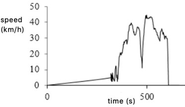
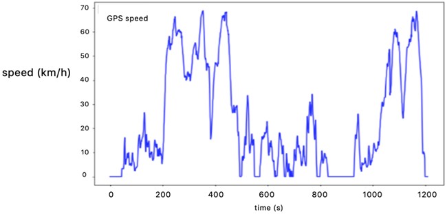
According to the transition probability matrix of category 1 and category 2, the driving condition of 1200 second typical road vehicle is synthesized by principal component analysis and K-means algorithm, shown in Fig. 9.

Fig. 9Representative driving condition curve of K-means clustering

4.2.3. K-means++ clustering results and analysis

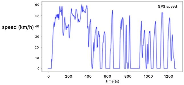
According to the transition probability matrices of category 1 and category 2, the principal component analysis-K-means++ method is used to synthesize a typical road driving condition map for 1200 seconds, as shown in Fig. 10. The traffic congestion in category 1 takes 824 seconds, while Category 2 is 381 seconds under relatively smooth conditions.

Fig. 10Representative driving conditions of K-means++ clustering

4.3. Comparative analysis of effectiveness

4.3.1. Comparative analysis of operating characteristics

The feature parameters such as $V_{m}$ (km/h), $V_{m r}$ (km/h), $A_{m}$ (m/s²), $D_{m}$ (m/s²), $P_{i}$ (%), $P_{a}$ (%), $P_{d}$ (%), $P_{c}$ (%), $V_{s}$ (km/h), $A_{s}$ (m/s²) are selected to evaluate the effectiveness of automobile motion characteristics the same as the operating condition curve constructed by PCA-K-means. Then it is compared and analysed between the representative construction conditions of the final construction and the sample parameters, in the end the error rates are calculated respectively (see Table 7).

Table 7Error probability analysis of K-means++ construction conditions relative to sample data

Characteristic parameters	Test data	PCA-K-means combination model		PCA-K-means++ combination model
Characteristic parameters	Test data	PCA-K-means	Error	PCA-K-means++	Error
$V_{m}$	16.481	16.995	3.12%	16.515	0.21%
$V_{m r}$	22.497	24.585	9.28 %	23.620	4.99 %
$V_{s}$	11.462	12.237	6.76 %	11.884	3.68 %
$A_{m}$	0.545	0.590	8.34 %	0.572	5.02 %
$D_{m}$	0.543	0.593	9.12 %	0.580	5.75 %
$A_{s}$	0.749	0.773	3.25 %	0.755	0.74 %
$P_{i}$	0.224	0.236	5.43 %	0.231	3.26 %
$P_{a}$	0.285	0.303	6.21 %	0.296	3.70 %
$P_{d}$	0.292	0.310	6.17 %	0.302	3.45 %
$P_{e}$	0.199	0.210	5.59 %	0.208	4.37 %

It can be seen from Table 7 that the error rate of representative working conditions and collected data constructed by PCA-K-means combination model is as high as 9 % and the minimum error rate is more than 3%; while the one constructed by PCA-K-means++ combination model is less than 6 %, and the error rate of some parameters (such as average speed and acceleration standard deviation) is less than 1 %. This fully shows that the statistical distribution characteristic parameters and driving condition proportion distribution law constructed by PCA-K-means++ combination model are consistent with the collected data, which are obviously higher than the working condition error rate constructed by PCA-K-means algorithm. It can be seen that the application of PCA-K-means++ combined model to build driving condition can better reflect the distribution of collected data in each speed segment, significantly improve the accuracy of driving condition construction and can more accurately reflect the driving state of a city vehicle, with stronger reliability.

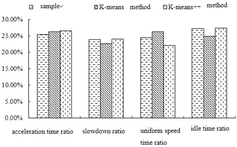
Taking speed frequency as an example, the paper compares and analyzes the distribution of vehicle driving state (Fig. 11). K-means and K-means++ methods have less error with sample data in reflecting vehicle driving state. However, the error rate between the representative working conditions constructed by K-means++ algorithm and the overall collected data is smaller, especially the proportion of deceleration time and idle time. Therefore, it can be considered that the driving condition constructed by K-means++ method is more suitable for local needs and can reflect the actual driving characteristics of local vehicles. It has certain theoretical and practical value for performance calibration of fuel consumption and emission.

Fig. 11Proportion distribution of vehicle driving conditions

4.3.2. Correlation analysis

The correlation coefficient between the representative working condition curve and the sample data curve constructed by PCA-K-means and PCA-K-means++ combination model was calculated respectively, shown in Table 8.

Table 8Comparison of correlation coefficients

Model	Correlation coefficient
PCA-K-means combination model	0.9276
PCA-K-means++ combination model	0.9684

The results show that the correlation coefficient between the representative working condition curve constructed by PCA-K-means combination model and sample data is 0.9276, while the one constructed by PCA-K-means++ combination model and sample data is 0.9684. Compared with PCA-K-means++ combination model, the correlation degree between driving condition curve and sample data is higher, which is 4.08 % higher than that of PCA-K-means. Therefore, PCA-K-means++ combination model can better reflect the actual driving level and road traffic characteristics of vehicles on the road.

5. Conclusions

In this paper, taking a city in China as an example, the real-time track of the same vehicle in two months is recorded, and a total of 496014 driving data are obtained.

1) In order to make the data accurate and reasonable, MATLAB software is used to preprocess the original data. Through interpolation of discontinuous data, screening and elimination of abnormal data, burr data processing and other operations, 457550 pieces of effective vehicle driving data are finally obtained. Python programming is used as well to divide the big data into micro stroke, the preprocessed data is divided into kinematic segments. A total of 3020 kinematic segments are obtained. After several selections of different number of feature parameters as principal component analysis, 16 feature parameters are selected to describe the operation conditions of all kinematic segments and 22 feature parameters are used to describe the overall distribution characteristics of kinematic segments. Besides, principal component analysis and K-means++ clustering algorithm are used to reduce dimension and classify the characteristic parameter matrix, so as to construct a vehicle driving condition of 1200 s in accordance with the traffic characteristics of a city.

2) Compared with the traditional K-means clustering algorithm, the vehicle driving condition model constructed by K-means++ algorithm can effectively solve the problem of unstable initial centre point and improve the accuracy of driving condition construction. It is found that the average relative error of driving condition generated by K-means++ algorithm is less than 6 %, the standard deviation error rate of average speed and acceleration is less than 1 %. The ratio of deceleration time to idle time is smaller in the running state of the vehicle. At the same time, the correlation between the vehicle driving condition curve and the sample data is higher than 4.08 %, which verifies the accuracy and effectiveness of the K-means++ clustering algorithm. Therefore, compared with NEDC, the driving condition constructed by K-means++ algorithm is more suitable for local needs and can reflect the actual driving characteristics of local vehicles. It has a certain theoretical and practical value for the calibration of vehicle fuel consumption, emissions and other performance indicators

3) Through the successful construction of the vehicle driving condition suitable for a certain city, it can provide certain reference for the construction of the actual driving characteristics of vehicles in other cities.

References

Cai Yan, Li Yangyang, Li Chunming, Tan Xiaowei, Liu Dongmin Research on synthetic technology of vehicle driving conditions in Xi’an based on K-Means clustering algorithm. Automobile Technology, Vol. 8, 2015, p. 33-36.

Search CrossRef
Qin Datong, Zhan Sen, Qi Zhenggang, Chen Shujiang Construction method of driving conditions based on K-means clustering algorithm. Journal of Jilin University (Engineering and Technology Edition), Vol. 46, Issue 2, 2016, p. 383-389.

Search CrossRef
Shi Qin, Qiu Duoyang, Zhou Jieyu Driving condition construction and accuracy analysis based on combined clustering method. Automotive Engineering, Vol. 34, Issue 2, 2012, p. 164-169+158.

Search CrossRef
Gao Jianping, Wu Jianguo Construction of vehicle driving conditions based on global K-means clustering algorithm. Journal of Henan University of Science and Technology (Natural Science), Vol. 38, Issue 1, 2019, p. 112-118.

Search CrossRef
Shi Qin, Zheng Yubo, Jiang Ping Research on driving conditions of urban roads based on kinematics segments. Automotive Engineering, Vol. 33, Issue 3, 2011, p. 256-261.

Search CrossRef
Knez M., Muneer T., Jereb B., et al. The estimation of a driving cycle for Celjeanda comparison to other European cities. Sustainable Cities and Society, Vol. 11, 2014, p. 56-60.

Publisher
Lin J., Niemeier D. A. Exploratory analysis comparing a stochastic driving cycle to California’s regulatory cycle. Atmospheric Environment, Vol. 36, Issue 38, 2002, p. 5759-5770.

Publisher
Liu Ye, Wu Sheng, Zhou Haihe, Wu Xingyi, Han Linyi Research on K-means clustering algorithm optimization method. Information Technology, Vol. 43, Issue 1, 2019, p. 66-70.

Search CrossRef
Li Yang Research on Car Driving Conditions Based on Clustering Algorithm. Beijing Institute of Technology, 2016.

Search CrossRef
Tian Yu Construction and Analysis of Road Driving Conditions for Light Vehicles in Taiyuan City. Taiyuan University of Technology, 2018.

Search CrossRef
Zhang Zhiyong, et al. Master of MATALB. Beijing University of Aeronautics and Astronautics Press, Beijing, 2011.

Search CrossRef
Sun Qiuyue, Wang Lizhen, Wu Fengping Introduction and application of data compression method. Journal of Yunnan University (Natural Science Edition), Vol. 29, Issue 1, 2007, p. 115-118.

Search CrossRef
Ma Zhixiong, Li Mengliang, Zhang Fuxing, et al. Application of principal component analysis to the development of vehicle actual driving conditions. Journal of Wuhan University of Technology, Vol. 26, Issue 4, 2004, p. 32-35.

Search CrossRef
Ai Guohe, Qiao Weigao, Li Mengliang, et al. Analysis of the kinematic parameters of vehicle driving. Highway Communications Science and Technology, Vol. 23, Issue 2, 2006, p. 154-157.

Search CrossRef
Shi Shuming, Wei Shuying, Hai Linkui, Liu Liu Improvement soft the design method for transient driving cycle for passenger car. IEEE Vehicle Power and Propulsion Conference, 2009, p. 1581-1586.

Publisher

Cited by

Research on Brake Energy Recovery Strategy Based on Working Condition Identification

Weiguang Zheng | Haiqiao Li | Jun Li

(2024)

Identifying Key Training Load and Intensity Indicators in Ice Hockey Using Unsupervised Machine Learning

Vincenzo Rago | Tiago Fernandes | Magni Mohr

(2024)

Working cycle condition construction for electric wheel loader based on principal component analysis and cluster analysis

(2024)

2024 12th International Conference on Traffic and Logistic Engineering (ICTLE)

(2024)

A dynamic competitive velocity prediction method based on Markov state space reconstruction

Rong Wang | Yan Ti | Xianrang Shi | Tinglun Song

(2024)

A novel construction and evaluation framework for driving cycle of electric vehicles based on energy consumption and emission analysis

Jianhua Guo | Dong Xie | Yu Jiang | Yue Li

(2024)

Review of Energy Management Methods for Fuel Cell Vehicles: From the Perspective of Driving Cycle Information

(2023)

Energy Management Strategy for Plug-In Hybrid Electric Vehicles Based on Driving Condition Recognition: A Review

Chunna Liu | Yan Liu

(2022)

A Neural Network and Principal Component Analysis Approach to Develop a Real-Time Driving Cycle in an Urban Environment: The Case of Addis Ababa, Ethiopia

Amanuel Gebisa | Girma Gebresenbet | Rajendiran Gopal | Ramesh Babu Nallamothu

(2022)

Research on Energy Consumption Generation Method of Fuel Cell Vehicles: Based on Naturalistic Driving Data Mining

Yangyang Ma | Pengyu Wang | Bin Li | Jianhua Li

(2022)

About this article

Received

27 April 2020

Accepted

09 August 2020

Published

30 September 2020

DOI

https://doi.org/10.21595/jme.2020.21433

Keywords

PCA-K-means++

driving condition

kinetic fragments

urban roads

light vehicles

This is an open access article distributed under the Creative Commons Attribution License, which permits unrestricted use, distribution, and reproduction in any medium, provided the original work is properly cited.

Previous article in issue Previous Next article in issue Next

Research article

2022 06 30

Nonlinear dynamic analysis of constant-speed and variable-speed of autonomous vehicle passing uneven road

Zhiyong Yang, Long Wang, Fangtao Liu, Zijian Li

Research article

2020 10 19

A sensor fault diagnosis method based on KPCA and contribution graph

Yuanqing Wang, Fan Deng

Research article

2019 11 28

PCA based health indicator for remaining useful life prediction of wind turbine gearbox

Hemanth Mithun Praveen, Divya Shah, Krishna Dutt Pandey, Vamsi I, Sabareesh G R

Research article

2019 04 25

Remaining useful life (RUL) prediction of bearing by using regression model and principal component analysis (PCA) technique

Apakrita Tayade, Sangram Patil, Vikas Phalle, Faruk Kazi, Satvasheel Powar

S. Guo, K. Wu, and G. Zhang, “Application of PCA-K-means++ combination model to construction of light vehicle driving conditions in intelligent traffic,” Journal of Measurements in Engineering, Vol. 8, No. 3, pp. 107–121, Sep. 2020, https://doi.org/10.21595/jme.2020.21433

Copy Extrica

Copied to clipboard!

TY  - JOUR
DO  - 10.21595/jme.2020.21433
UR  - https://doi.org/10.21595/jme.2020.21433
TI  - Application of PCA-K-means++ combination model to construction of light vehicle driving conditions in intelligent traffic
T2  - Journal of Measurements in Engineering
AU  - Guo, Shuqing
AU  - Wu, Kangkai
AU  - Zhang, Guoqing
PY  - 2020
DA  - 2020/09/30
PB  - JVE International Ltd.
SP  - 107-121
IS  - 3
VL  - 8
SN  - 2335-2124
SN  - 2424-4635
ER  - 

Copy Ris

Copied to clipboard!

@article{Guo_2020,
	doi = {10.21595/jme.2020.21433},
	url = {https://doi.org/10.21595/jme.2020.21433},
	year = 2020,
	month = {sep},
	publisher = {{JVE} International Ltd.},
	volume = {8},
	number = {3},
	pages = {107--121},
	author = {Shuqing Guo and Kangkai Wu and Guoqing Zhang},
	title = {Application of {PCA}-K-means$\mathplus$$\mathplus$ combination model to construction of light vehicle driving conditions in intelligent traffic},
	journal = {Journal of Measurements in Engineering}
}

Copy Bibtex

Copied to clipboard!

[1]S. Guo, K. Wu, and G. Zhang, “Application of PCA-K-means++ combination model to construction of light vehicle driving conditions in intelligent traffic,” Journal of Measurements in Engineering, vol. 8, no. 3, pp. 107–121, Sep. 2020, doi: 10.21595/jme.2020.21433.

Copy IEEE

Copied to clipboard!

Guo, Shuqing, Kangkai Wu, and Guoqing Zhang. “Application of PCA-K-Means++ Combination Model to Construction of Light Vehicle Driving Conditions in Intelligent Traffic.” Journal of Measurements in Engineering 8, no. 3 (September 30, 2020): 107–21. https://doi.org/10.21595/jme.2020.21433.

Copy Chicago

Copied to clipboard!

Application of PCA-K-means++ combination model to construction of light vehicle driving conditions in intelligent traffic

Abstract

1. Introduction

2. Model approach

2.1. Kinematic fragment

2.2. Principal component analysis

2.3. K-means++ clustering method

2.3.1. K-means++ algorithm theory

2.4. Correlation analysis

3. Data acquisition and processing

3.1. Data collection

3.2. Data pre-processing

3.2.1. Intermittent data processing

3.2.2. Acceleration and deceleration abnormal data processing

3.2.3. Idle abnormal data processing

3.2.4. Glitch data processing

3.2.5. Long idle time abnormal data

4. Construction of driving condition model and result analysis

4.1. Kinematic segmentation

4.2. Construction of driving conditions model

4.2.1. PCA analysis results

4.2.2. K-means clustering results and analysis

4.2.3. K-means++ clustering results and analysis

4.3. Comparative analysis of effectiveness

4.3.1. Comparative analysis of operating characteristics

4.3.2. Correlation analysis

5. Conclusions

References

Cited by

About this article

Related Articles