Solving the problem of moving a solid body around a fixed point in a resisting medium

1. Introduction

The problem of motion of a solid body with a fixed point is one of the remarkable problems of classical mechanics. The peculiarity of this problem is that, despite the important results obtained by the largest mathematicians over the past two centuries, there is still no complete solution [1-4]. Mathematically, these problems are reduced to the study of a system of nonlinear differential equations and differential equations with variable coefficients, obtaining analytical solutions to which is extremely difficult and is possible in a relatively small number of cases. Therefore, the construction of analytical solutions for a wide class of such problems is very relevant.

In this paper, an analytical solution of the problem is obtained by a new method called the partial discretization method. The method is based on generalized functions [5]. Using the partial discretization method, it is easy to obtain an analytical solution of nonlinear differential equations or differential equations with variable coefficients. One of these equations is the dynamic Euler equations, which describes the movement of a solid body around a fixed point in a resisting medium.

Using the method of partial discretization of nonlinear differential equations based on the theory of generalized functions, an analytical solution to the problem of the movement of a solid body around a fixed point in a resisting medium is obtained, which is described by the nonlinear dynamic equations of L. Euler.

2. Materials and methods

Consider the nonlinear dynamic equations of L. Euler [6], which describe the movement of a solid body around a fixed point in a resisting medium:

where $A$, $B$, $C$ – moments of inertia of the body relative to the axes $x$, $y$, $z$ associated with the body; $p$, $q$, $r$ – projections of the angular velocity vector of a body on these axes; $M_x$, $M_y$, $M_z$ – moments of external resistance forces relative to the axes $x$, $y$, $z$.

The system of differential Eq. (1) is considered together with the initial conditions:

Without limiting the generality of the problem, we will assume that:

Let the moments of external forces are created only by forces of some resistance and are linearly proportional to the corresponding projections of the angular velocity of the body:

where ${\lambda }_1$, ${\lambda }_2$, ${\lambda }_3$ – custom parameters that depend on the environment properties. We turn to the case of a symmetric solid when $A=B$. Then the system of nonlinear differential Eq. (1) taking into account the initial conditions Eqs. (2), (3) will take the form:

where:

From system Eq. (5) to determine the projection $p\left(t\right)$ of the angular velocity of a body, we have the following differential equation with variable coefficients:

To solve the problem Eq. (7) – Eq. (2), Eq. (3), applying the method of partial discretization of nonlinear differential equations [7], we obtain:

where $\delta \left(t\right)$ – delta function of Dirac.

The General solution of Eq. (8) has the expression:

where $H\left(t\right)$ – the function of Heaviside; $C_1$ and $C_2$ – arbitrary constant of integration.

Using the initial conditions Eqs. (2) and (3), we have:

According to Eq. (10), expressions of the function $p\left(t\right)$ at points $t_i\left(i=\overline{1,n}\right)$ are written as follows:

Fig. 1 show graphs of problem solving for various parameter values. In some cases, the solutions are compared with previously obtained literary solutions, which show a complete coincidence of the integral curves.

3. Results and discussion

The General solution of Eq. (7), expressed in terms of Bessel functions, is obtained by V. N. Koshlyakov [6, p. 72] as:

where $\nu =-\frac{1}{2}+\frac{C}{2A}\frac{{\lambda }_1-{\lambda }_2}{{\lambda }_3}$.

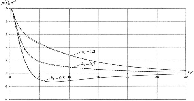
Figs. 1, 2 shows graphs comparing curves for the case ${\lambda }_1={\lambda }_2$ with the solution obtained by corresponding member of the USSR Academy of Sciences V. N. Koshlyakov in Bessel functions. Solid lines show curves drawn in accordance with the solution Eq. (10), and dotted lines Eq. (12).

Fig. 1Graph velocity projection pt change curves for parameter values: A= 10 kg⋅m2, C= 20 kg⋅m2, p0= 10 sec-1, r0= 1 sec-1, λ1=λ2= 0,2. - - - - - - the solution obtained By V. N. Koshlyakov, __________ the solution received by the author

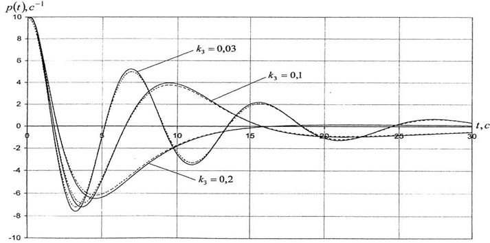
Fig. 2Graph velocity projection pt change curves for parameter values: A= 10 kg⋅m2, C= 20 kg⋅m2, p0= 10 sec-1, r0= 1 sec-1, λ1=λ2= 0,2. - - - - - - the solution obtained By V. N. Koshlyakov, __________ the solution received by the author

4. Conclusions

Analysis of the results showed that a significant resistance of the medium (Fig. 2) encourages the gyroscope to smooth unidirectional movement with slow attenuation, while relatively small resistances (Fig. 1) do not interfere with the oscillatory process, causing alternating movements of the object under consideration. The results of this work are a great contribution to the theory of gyroscopes and gyroscopic systems and can be used in the development of new stabilizing elements of various inertial navigation systems on ships, aircraft, missiles, satellites and spacecraft [8].

References

-
Amer Tarek, Abady I. M. Solutions of Euler’s dynamic equations for the motion of a rigid body. Journal of Aerospace Engineering, Vol. 30, Issue 4, 2017, p. 04017021.
Ershkov S. V. New exact solution of Euler’s equations (rigid body dynamics) in the case of rotation over the fixed point. Archive of Applied Mechanics, Vol. 84, 2014, p. 385-389.
Tsiotras Panagiotis, Longuskiy James M. Analytic solution of Eulers equations of motion for an asymmetric rigid body. ASME Journal of Applied Mechanics, Vol. 63, Issue 1, 1996, p. 149-155.
Bohner Martin, Peterson Allian First and second order linear dynamic equations on time scales. Journal of Difference Equations and Applications, Vol. 7, Issue 6, 2001, p. 767-792.
Vladimirov V. S. Generalized functions and their application. Knowledge, Moscow, 1990.
Koshlyakov V. N. Problems of Rigid Body Dynamics and Applied Gyroscope Theory: Analytical Methods. Russian. Nauka, Moscow, 1985, p. 286.
Tyurekhojayev A. N., Mamatova G. U. Analytic solution of differential equation for gyroscope’s motion. International Conference on Analysis and Applied Mathematics, 2016.
Awrejcewicz Jan, Koruba Zbigniew Classical Mechanics: Applied Mechanics and Mechatronics. Springer, New York Heidelberg Dordrecht London, 2012.
About this article