Abstract
Using objective vibration evaluation to produce results highly consistent with real road ride comfort is challenging. The deficiencies in traditional evaluation indices, adopting an average operator, maximum operator, or cumulative operator as the main vibration information integration logic, are reported here through 19 designed road field tests in which major vibration information distribution covers all axes and vibration information is distributed in spacetime in various patterns. A new evaluation index which adopted a combination of maximum and cumulative operator is proposed to overcome these deficiencies and an interactive mechanism which standardized the process of selecting vibration information distributed among axes and spacetime is devised between the localized major vibrations. The results show that the proposed road ride comfort evaluation index is more consistent and accurate than the evaluation indices proposed by ISO 2631-1 and can be used more generally.
1. Introduction
People in commuter or industrial vehicles are exposed to various types of whole-body vibrations. These vibrations can lead to feelings of discomfort, which are not merely unpleasant, but are also related to health risks [1]. Whole-body vibrations can lead to harmful effects in the cardiovascular, musculoskeletal, and central nervous systems, as well as other areas of the human body [2, 3]. Therefore, evaluating these vibrations is crucial, and vibration reduction methods can be developed based on that, such as an optimization design method for a body mounting system developed by Liu et al. [4] and an optimization scheme for the powertrain mount system of an electric vehicle proposed by Xin et al. [5]. The success of those vibration evaluation methodologies rely heavily upon their accuracy and applicability; however, a lack of sufficient theoretical and practical support has led to inaccurate and even contradictory evaluation results compared to true values. This is a problem because recent investigations in the automobile industry revealed that customers are expressing greater needs in terms of improved road ride comfort [6], and a prerequisite to successfully meeting their needs is an appropriate evaluation.
Current road ride comfort evaluation methods were established based on laboratory test results, partly because the test conditions are likely to be strictly controlled, so the results are more comparable. Evidence shows that field tests do not produce independent major vibration information for the longitudinal, lateral, vertical, roll, pitch, and yaw axes, complicating analyses [7, 8]. As such, few evaluation methods have been established based on field test results, and this is increasingly becoming a problem. Laboratory tests mostly adopt consecutive sinusoidal excitation as the input, whereas most excitations in actual field tests are non-sinusoidal and non-consecutive – they are random or quasi-random [9, 10], so the suitability of directly applying laboratory-based methods to actual field test scenarios is in doubt. Mansfield et al. [11] found that the correlation strength between several vibration evaluation methods and normalized subjective discomfort scores is strongly influenced when excitation type changes from non-random to random or quasi-random. Dickey et al. [12] showed that different combinations of major vibration axes can lead to different levels of discomfort, which is not captured by current methodologies. How actual field test results differ from laboratory based theoretical predictions needs to be investigated in more depth.
Specifically, the road ride comfort evaluation indices can be divided into subjective and objective indices. The subjective evaluation indices require a scoring scale and corresponding semantic levels; a group of people assign their subjective scores after being exposed to vibrations in actual road field tests, then the scores are processed to form a unique value that represents road ride comfort. Subjective indices are generally accurate and are regarded as the true value of road ride comfort because they provide a direct output of human experience. When employing subjective methods, a minimal number of people must be involved to ensure statistical stability. The American Society of Testing Materials (ASTM) specifies a rating panel size of 15 members based on a 0.3 mean panel rating (MPR) maximum error with a normal distribution [13]. Nakamura found that the evaluation results by the American Association of State Highways Officials (AASHO) subjective scoring method deviate from true values by more than 0.4 units in less than 5 % possibility when the number of participants reaches 20 [14]. People who participate in the test must also be representative of the population in terms of age, sex, and other factors so the results will be more representative. These requirements mean subjective methods are time consuming and expensive, and are therefore unable to be scaled up for large-scale use. Subjective methods are a black box process; the quantitative relationship between objective vibration information and subjective scores is unclear, so they cannot directly provide further guidance for health risk prevention.
Objective evaluation indices are more widely used because they involve a white box process, and the data collection and processing are performed more automatically, which lowers the cost. Objective evaluation indices typically integrate vibration information in the entire timeline or frequency zone to represent real road ride comfort; the integration methods vary and lead to different results. First, an average operator is adopted as the main logic to integrate vibration information. The international roughness index (IRI) is defined as the cumulative displacement of the suspension system when a standard vehicle travels 1 km at a speed of 80 km h−1 [15]; it is transformed to create ride quality indexes (RQI), such as China RQI [16] and Minnesota RQI [17]. IRI has its own deficiencies: (1) it is based on displacement, whereas ride comfort is more related to acceleration or other physical quantities [18-20]; and (2) the human body is sensitive to wavelengths between 0.5 and 2.5 m [21]. IRI is sensitive to wavelengths between 2.4 and 15 m [22]; therefore, it cannot appropriately reflect human response to vibration frequencies. IRI normalizes the integration interval to 1 km irrespective of the real interval, so its integration mechanism uses an average operator. Root mean square (RMS) [23] values of frequency weighted acceleration and average absorbed power (AAP) [24] also adopt this average logic. Griffin [25] suggested that using an average operator in the time zone is oversimplistic because it can result in excessive estimation for short durations or apparently unreasonably low estimation for long durations; periods containing different magnitudes, transients, and shocks in varying vibration exposure must be defined. Standardizing the total integration time can solve this problem, but it is almost impossible to achieve [10, 26]. Secondly, a maximum operator is adopted as the main logic to integrate vibration information. The maximum transient vibration value (MTVV) is a typical example; it only integrates the largest vibration information within one second [23]. However, the vibration information beyond the maximum one second part can also significantly affect human discomfort, so MTVV is unsuitable [2, 11]. Vibration greatness (VG), proposed by Miwa [27], integrates vibration information beyond the maximum part, but the integration process is purely in the frequency domain, which is inevitably accompanied by a loss of information on location and geometric characteristics for transients that are essential for evaluating road ride comfort [28]. Thirdly, a cumulative operator is adopted as the main logic to integrate vibration information. Indices using this logic only increase when new vibration information is introduced and thus do not suffer from large shifts due to total integration time alone. Vibration dose value (VDV) is a typical example and is currently considered a good index because its high integration order of four is deemed to appropriately consider shocks, which is based on frequency weighted acceleration capable of representing human response to frequencies [11, 29]. Griffin [26] stated that there is currently no evidence to suggest a measure that is more accurate than VDV. Total absorbed power [30] and total daily acceleration dose [31] also adopt a cumulative operator as the main vibration information integration logic. Total absorbed power does not need frequency weightings because it is energy-based. The total daily acceleration dose only considers vibration in the vertical axis and can only provide guidance for spinal risk prevention. Indices using a cumulative operator to integrate vibration information in the time domain are at risk of over integration. For example, adults may suffer considerable vibrations during their lifetime when riding in vehicles. Although this means that the calculation results for these indices are high, the passenger may not currently feel uncomfortable. The International Standard Organization (ISO) specifies that the VDV and total daily acceleration dose should be limited in a whole day, which suggests that the longer the vibration exposure, the more inaccurate the two indices. Fourth, a combination of different operators is adopted as the main logic to integrate vibration information. Weighted longitudinal profile (WLP) uses a combination of variance and range to evaluate road ride comfort [28]; however, it cannot completely avoid the deficiencies of both operators. One variance can correspond to infinite combinations of wavelengths and amplitudes, which can lead to diverse levels of road ride comfort [32]. This is also the case even if a peak value is fixed. As such, determining how vibration information should be integrated to better represent real road ride comfort is a problem to be overcome.
In this study, we aimed to establish a more general objective road ride comfort evaluation index. When applied to various road field test scenarios, the proposed index is consistent and accurate. This process is based on field test results, which are deemed to more accurately represent actual situations. The designed scenarios cover major vibration information in all axes because the current trend is to use multi-axis vibration information [33, 34]. The main findings are that localized major vibrations and their interactions, rather than all vibration information, should be integrated to appropriately represent road ride comfort, and the interactive forms vary according to localized characteristics.
2. Materials and methods
2.1. Field test configurations
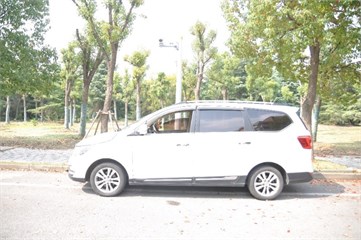
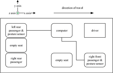
A subjective scoring method was developed in this research. Considering the accuracy required in the analysis and the operational ease, the scoring scale was designed as shown in Fig. 1. Only 4 semantic levels are involved, and the minimal interval is 0.1. The objective vibration data were collected by JY-901-type or HWT-901B-type posture sensors (Witmotion, Shenzhen, China). They collect the same vibration information; the difference is that the data transmission line is fixed to the latter, thus lowering the risk of connection failure. The posture sensors collect translational axis acceleration (m s−2), rotational angular velocity (rad s−1), and rotational angles (rad) in the , , and directions at a frequency of 200 Hz. The sensors were attached to the central surface of the seat of a Baojun-730-type test vehicle (SACI-GM, Shanghai, China) using Fixate gel pads (Frosted Concepts, Bristol, Australia). The test vehicle and its layout are shown in Fig. 2. The vibration information collected by the posture sensor in the right front seat also represents the information in the right rear seat. The sensors were inertial type and set onto an inclined surface, and adopted a Tait-Bryan coordinate system. The actual directly used vibration information was calculated using Eq. (1):
where , , , , , and are the actual used accelerations in the , , and axis and rotational angular velocities in the , , and axis in moment , respectively. The above variables with a subscript 0 directly represent the corresponding vibration information output directly by the posture sensors. , and are the rotational angles in , , and axis of the Tait-Bryant coordinate system, respectively; is the local gravitational acceleration. The installation ensures 0, whereas , , and g were chosen as the recorded maximum density value of the angle in the and axes, output directly by the posture sensors, and acceleration in the axis after the treatment in the right of Eq. (1), respectively.
Fig. 1Subjective scoring scale
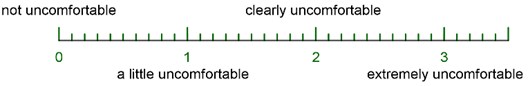
Fig. 2Test vehicle and its layout: a) Baojun 730-type test vehicle; b) layout in the test vehicle
a)
b)
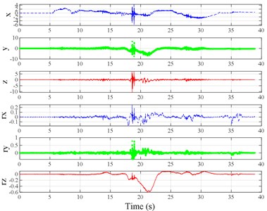
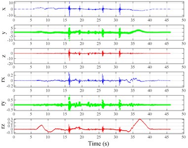
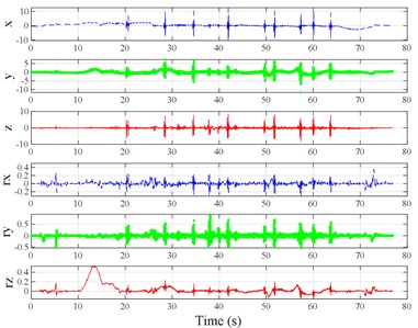
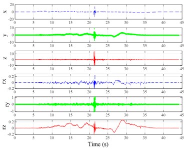
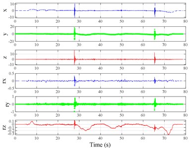
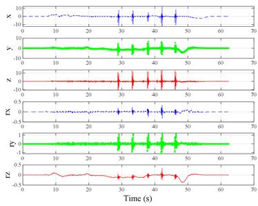
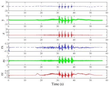
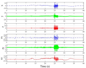
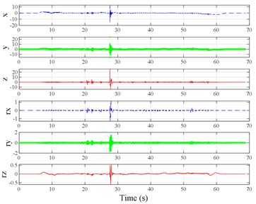
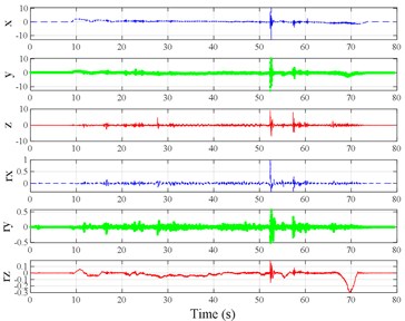
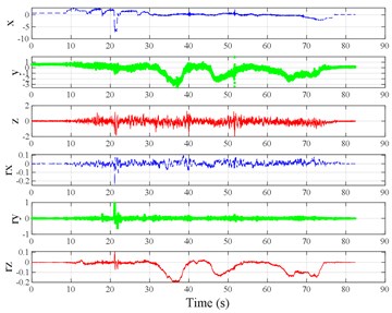
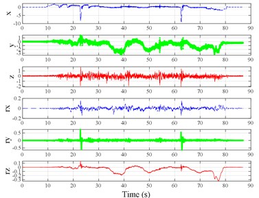
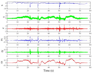
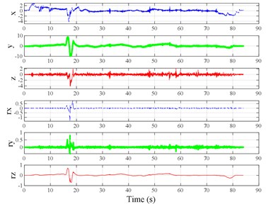
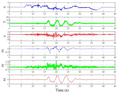
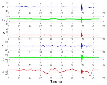
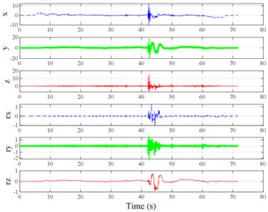
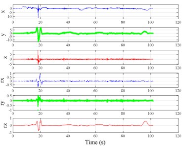
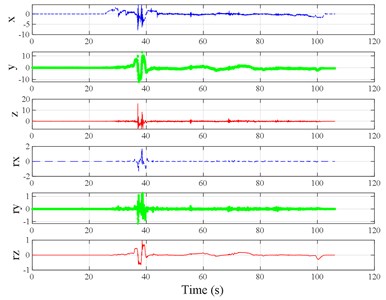
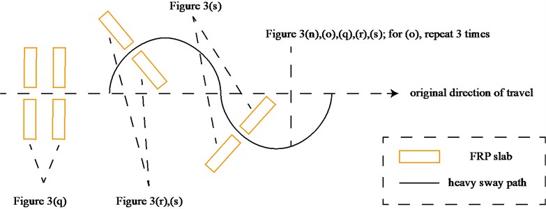
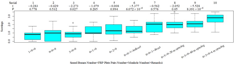
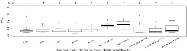
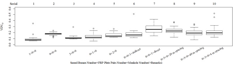
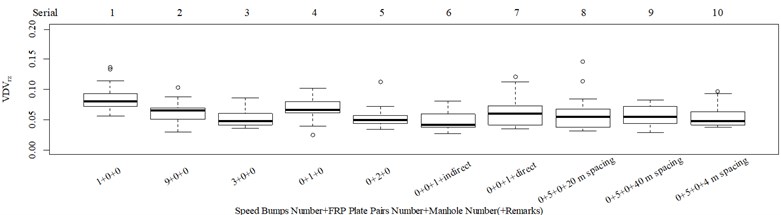
The test scenarios were divided into 4 groups. The scenarios in the first, second, and third group were deemed as producing major translational vibration information only in the , , or axis, respectively. Scenarios in the fourth group were deemed as producing major vibration information in more than one translational axis. Vibration information productions in the rotational axes were not especially designed, they occur with vibration information in the translational axes. Fig. 3 shows , , , , , and in the designed scenarios. The first group is shown in Fig. 3(a-j). The speed bumps in scenarios represented by Fig. 3(a-c) were trapezium-shaped, 110 mm in the upper base, 300 mm in the lower base, 45 mm high, and 3300 mm wide. Each FRP slab in scenarios represented by Fig. 3(d-h) was 300 mm in length, 55 mm high, and 1000 mm wide. Two FRP slabs formed a pair that was crossed by the test vehicle simultaneously. Fig. 3(i, j) show the scenarios of crossing an abnormally raised manhole, only wheels on one side crossed the manhole, this side was called the directly crossing side, the other side was called the indirectly crossing side. The second group is shown in Fig. 3(k-m), the third group is shown in Fig. 3(n, o), and the fourth group is shown in Fig. 3(p-s). The schemes in Fig. 3 (n, o, q–s) are shown in Fig. 4. In these designed scenarios, our major considerations were to include as many excitation types and major vibrational axes and vibration information distribution characteristics as possible. ISO 2631-1 [23] or BS (British Standard) 6841 [35] adopt the crest factor, defined as peak value divided by RMS, as a judgement index for choosing a specific ride comfort evaluation index, suggesting that the vibration information distribution characteristics essentially affect the performances of the indexes. Therefore, the spacing between excitations and the number of excitations is considered. Note that the vibration information shown in Fig. 3 is only a representative; it might not be reproduced precisely because the movements were conducted manually by the drivers. Vibration information on only one side is provided because symmetry characteristics were designed; the exceptions are the scenarios represented by Fig. 3(i, j), where they are highly asymmetric.
Fig. 3Vibration information in designed scenarios: a)-c) Crossing 1, 3, and 9 speed bumps at the speed of 40 km h−1, respectively; d), e) crossing 1 and 2 fiber-reinforced polymer (FRP) slab pairs at 40 km h−1, respectively; f)-h) crossing 5 FRP slab pairs with 40, 20, and 4 m spacing at 40 km h−1, respectively; i)-j) directly and indirectly crossing 1 manhole at 50 km h−1, respectively; k)-m) enduring 1, 2, and 3 sudden halts at the speed of 40 km h−1, respectively; n) enduring 1 heavy sway at 40 km h−1; o) enduring 3 consecutive heavy sways at 40 km h−1; p) crossing 1 FRP slab pair and then immediately enduring 1 sudden halt from 40 km h−1; q) crossing 2 FRP slab pairs with 4 m spacing and then immediately enduring 1 heavy sway at 40 km h−1; r), s) enduring 1 heavy sway and simultaneously crossing 1 and 2 FRP slab pairs at 40 km h−1, respectively. The unit for translational axes is m s-2, the unit for rotational axes is rad s-1
a)
b)
c)
d)
e)
f)
g)
h)
i)
j)
k)
l)
m)
n)
o)
p)
q)
r)
s)
Each scenario was experienced by 27-35 people (average 32.895, 61.280 % men). The age range was 20-50 years (average 30.910 years). The height range was 153-183 cm (average 169.714 cm). The weight range was 42-105 kg (average 65.920 kg). The testing sequences are randomly assigned and the testers were not told what excitation would they experience to avoid the Hawthorne effect [36]. All subjects provided their informed consent for inclusion before they participated in the study. The study was conducted in accordance with the Declaration of Helsinki, and the protocol was approved by the Ethics Committee of Tongji University (2019tjdx294).
Fig. 4Excitation configurations schematic diagram for scenarios containing at least one heavy sway
2.2. Analysis of the road field test results
RMS, MTVV, VDV, and pseudo vibration total value (PVTV) were chosen as the reference road ride comfort evaluation indexes for the road field test. The calculation equations for RMS, MTVV, and VDV are shown in Eqs. (2-4), respectively [23]. The calculation equation for PVTV is shown in Eq. (5). The frequency weightings for these indexes are provided by ISO 2631-1, in which and axis, axis, and rotational axes respectively adopt a distinct frequency weightings. We chose these indexes because RMS, MTVV, VDV, and vibration total value (VTV) are currently widely used. RMS, MTVV, and VDV adopt an average operator, a maximum operator, and a cumulative operator as the main logic to integrate vibration information, respectively. VTV is a further development for RMS, which includes vibration information in the rotational axes, whereas RMS, MTVV, and VDV do not. These indexes are contradictory on this point but are included in the same ride comfort evaluation standard ISO 2631-1, this is another reason for why we put these indexes together for comparisons.
PVTV is different from VTV on the point that in the rotational axes it is based on frequency weighted rotational angular velocity rather than frequency weighted rotational angular acceleration. Using PVTV rather than VTV is because the posture sensors directly collect angular velocities, calculating angular accelerations directly from discrete angular velocities would lead to excessive large results. The alternatives for absolute balance weight in the rotational axis is chosen as 1 to 10 with an interval of 1, these alternatives do not allow the rotational axis contribution to exceed 50 %, as is suggested by ISO 2631-1. The optimal for PVTV is 1, and this parameter set PVTV is chosen for comparisons. The optimize model is chosen as recursive partitioning and regression trees (RPART) [37], the input is PVTV and testers, the output is subjective scorings. Testers were added to the input variables because different people respond largely to the same kind of vibration. Adding this variable can help to largely reduce the fitting errors [38]. For the RPART model, the minimum number of observations in a node for a split to be attempted was set to 20, any split that does not decrease the overall lack of fit by a factor of complexity parameter of 0.015 was not attempted, the maximum depth of any node of the final tree was set to 10 (the root node was counted as depth 0), and the number of cross-validations was set to 10. The normalized mean square error (NMSE) was chosen as the measurement of fitting errors, which is the main measurement of the performance of the objective evaluation indexes. The reference model for NMSE is the mean value model:
where is the momentum in axis at moment , which is frequency weighted acceleration in the translational axes or frequency weighted angular velocity in the rotational axes; is the total integration time; is the local integration time, its default value is 1 s; is any end moment; is the axial weight, where 1, 0.63, 0.4, 0.2; is the absolute balance weight in axis j, which is used to balance the weights between translational axes and rotational axes; we set 1 for standardizing purposes. , is the absolute balance weight in the rotational axis, 0. ISO only suggests the calculation for RMS, MTVV, and VDV in the translational axes, which we expanded to the rotational axes to enable comparison in this research.
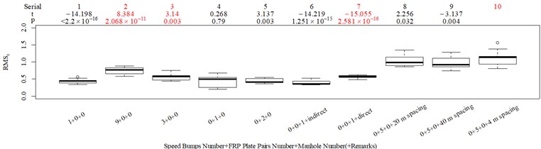
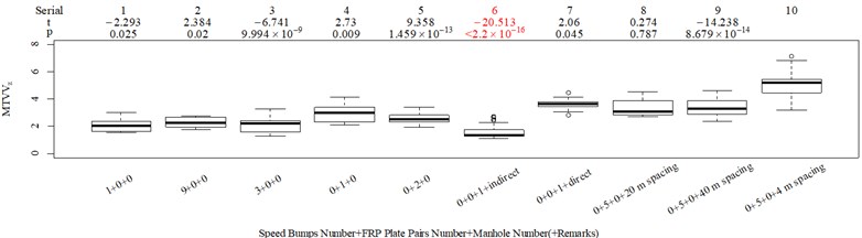
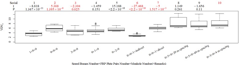
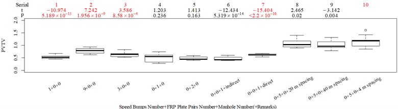
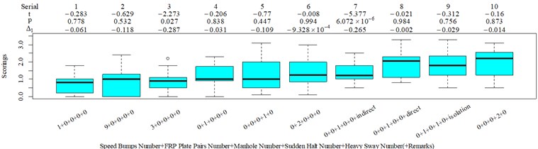
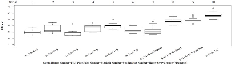
The subjective scoring results and objective evaluation results for groups 1, 2, 3, and 4 are shown in Fig. 5(a-e), (f-j), (k-o), (p-t), respectively. The values at the top of Fig. 5 are the -values and -values of a -test between the below column and the adjacent right column. The columns for subjective scoring results are arranged so that t-values are always lower or equal to 0; this column sequence was also applied to the corresponding objective evaluation results. Fig. 5 only shows the major vibration axis information; the exceptions are group 4 scenarios due to the multiple major vibrational axes. We ensured the other translational axes only contained minor vibration information and are not demonstrated in Fig. 5. The objective evaluation results in the rotational axes are also not provided independently in Fig. 5 because both ISO 2631-1 and BS 6841 suggest that using vibration information in the translational axes is sufficient.
Fig. 5Boxplot of subjective scoring results and objective evaluation results in the designed scenarios: a), f), k), p) the subjective scoring results for groups 1, 2, 3, and 4, respectively; b)-e) RMSz, MTVVz, VDVz, and PVTV for group 1, respectively; g)-j) RMSx, MTVVx, VDVx, and PVTV for group 2, respectively; l)-o) RMSy, MTVVy, VDVy, and PVTV for group 3, respectively; q)-s) RMSx, RMSy, RMSz for group 4, respectively; t)-v) MTVVx, MTVVy, MTVVz for group 4, respectively; w)-y) VDVx, VDVy, VDVz for group 4, respectively; and z) PVTV for group 4
a)
b)
c)
d)
e)
f)
g)
h)
i)
j)
k)
l)
m)
n)
o)
p)
q)
r)
s)
t)
u)
v)
w)
x)
y)
z)
The t-test results are described as: (1) when 0.05, there is no significant difference; (2) when 0.001 0.05, there is significant difference; (3) when 0.001, there is highly significant difference. Wasserstein and Lazar [39], on behalf of the American Statistical Association (ASA), stated that traditional thresholds for p-values are empirical and should not be strictly followed. In this case, when subjective scoring results and objective evaluation results are highly contradictory, we must comment; if we do not provide any comment, we use p-values as an auxiliary judging measure. The column sequence number and - values and -values in Fig. 5 are marked red when this column is suspected to have a major problem. The values in group 4, except for those in Fig. 5(z), are all marked green because the corresponding scenarios involve more than one major vibrational axis; therefore, using vibration information in only one axis to judge the total discomfort would be inappropriate.
RMS, MTVV, VDV, and PVTV performed poorly in some of the designed scenarios. For group 1, when compared to Fig. 5(a): (1) Fig. 5(b) shows RMS highly significantly over-integrated the vibration information in the scenarios represented by columns 2 and 3, and highly significantly under-integrated vibration information in scenarios represented by columns 7 and 10; (2) Fig. 5(c) shows MTVV produced evaluation results consistent with the subjective evaluation results except for highly significantly under-integrating the vibration information in the scenarios represented by column 7; (3) Fig. 5(d) shows VDV highly significantly over-integrated the vibration results in the scenarios represented by column 2 and 3, and highly significantly under-integrated vibration information in scenarios represented by columns 7, 8, and 10; (4) the - value and -value in the additional -test between columns 1 and 6 in Fig. 5(e) are 4.947 and 5.64×10⁻⁶, respectively. Therefore, Fig. 5(e) shows PVTV highly significantly over-integrated the vibration information in scenarios represented by columns 1-3, and highly significantly under-integrated the vibration information in the scenarios represented by columns 7 and 10.
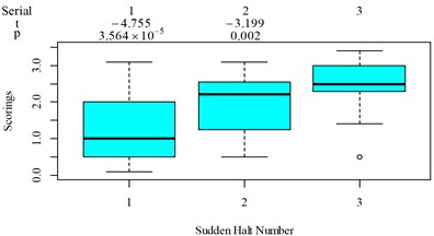
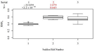
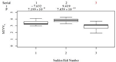
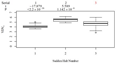
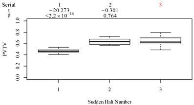
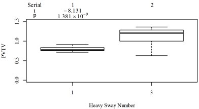
For group 2, the following contradictory evaluation results were obtained: (1) the subjective scorings in column 3 are significantly higher than in column 2, whereas the RMSx in column 3 is significantly lower than the RMSx in column 2; (2) the subjective scorings in column 3 are highly significantly higher than the subjective scorings in column 1, whereas the MTVVx in column 3 is highly significantly lower than the MTVVx in column 1 ( −5.058, 6.356 × 10⁻⁶); (3) the subjective scorings in column 3 are significantly higher than subjective scorings in column 2, whereas VDVx in column 3 is highly significantly lower than VDVx in column 2; (4) the subjective scorings in column 3 are significantly higher than subjective scorings in column 2, whereas there is no significant difference between the PVTV in columns 2 and 3.
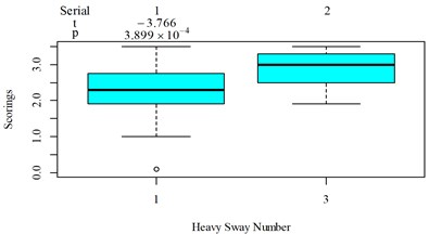
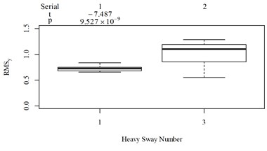
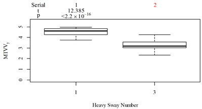
For group 3, when compared to Fig. 5(k): (1) MTVV highly significantly under-integrated the vibration information in the scenario represented by column 2; and (2) VDV highly significantly over-integrated the vibration information in the scenario represented by column 1.
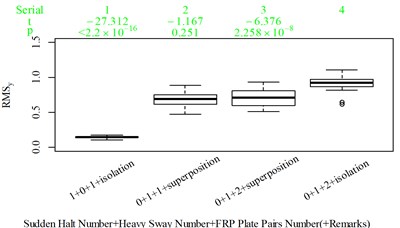
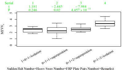
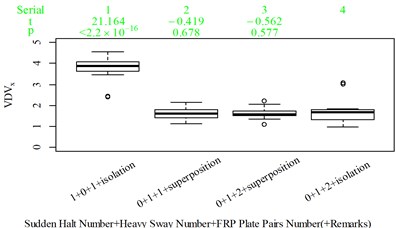
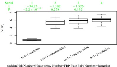
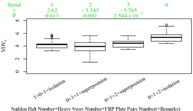
For group 4, the RMSy in column 4 is highly significantly higher than that in column 3, whereas we found no significant difference in MTVVy or VDVy between columns 3 and 4. The mechanism into these discrepancies must be interpreted, and a new road ride comfort evaluation index capable of overcoming these discrepancies needs to be developed to achieve better consistency and accuracy.
2.3. Establishing a new ride comfort evaluation index
Columns 1-3 in Fig. 5(a-e) provide the vibration information introduced by only one speed bump integrated to represent real discomfort; otherwise, over-integration occurs. So, the localized vibration information introduced by each speed bump was extracted first and then we decided which information was going to be integrated. Localized characteristics are essential for road ride comfort evaluation because vibration information distribution in an actual road riding process is often highly uneven [40, 41]. A local impact concept is proposed in the following steps to capture the major vibration information in localized segments:
1. Calculate translational axes energy density using:
2. Find a consecutive interval that covers the largest point in the residual timeline, can maximally integrate total , and is limited to a maximum length of local integration time τ. This procedure is shown in Eqs. (7) and (8):
where is the total translational axes energy for the th local impact; is the end moment for the th local impact, 0; and is the moment when in the residual timeline reaches its maximal value.
3. Remove the vibration information included in from the existing timeline.
4. If , on the condition that and decreasing factor , then proceed to step 5. Otherwise, set and return to step 2.
5. If any is lower than , delete this .
6. Rename the left from its emerging sequence to ensure the sequence starts from 1. With each time step, add 1, then the slice corresponding to is defined as the th local impact.
Steps 4 and 5 above were designed according to the Beibo law: when someone experiences a strong excitation, then other excitations become negligible [42].
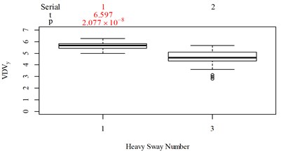
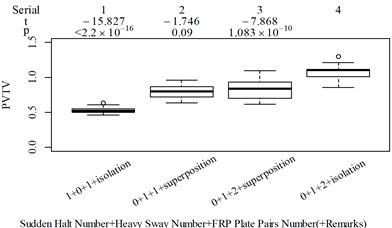
We found no significant difference between columns 4 and 5 in Fig. 5(a), which means the number of FRP slab pairs in these scenarios do not affect the total discomfort and is accordance with the results in columns 1-3 in Fig. 5(a, c). However, when the time spacing between FRP slab pairs is sharply reduced, as shown in Fig. 3(e, f), the total discomfort highly significantly increased, as shown in columns 5 and 9 in Fig. 5(a). So, localized major vibrations do not always individually represent total discomfort; they can interact with each other and add to total discomfort when their time spacings are short enough. In this case, a vibration perception window concept is proposed to quantify the conditional interactions between localized major vibrations, which assumes localized vibrations can interact with other vibrations within a limited time window. Columns 1 and 4 in Fig. 5(d) show that the vibration intensity produced by the FRP slab pair was higher than that produced by the speed bump. Fig. 3(c, f) show the time spacings between the FRP slab pairs were larger than those between the speed bumps, yet the FRP slab pairs were able to interact with each other and highly significantly add to total discomfort, whereas the speed bumps were not, as shown in columns 1 and 2 in Fig. 5(a), which suggests the FRP slab pair was able to interact with a wider range of vibration information than the speed bump. In this case, the window length was designed to increase with increasing localized vibration intensity, as shown in Eq. (9). Fig. 3(e, l) each contain the same two designed types of excitations the time spacings between the excitations in the two scenarios were designed to be the same. The vibration intensity represented by VDV in the main vibration axis was also not significantly different, as shown in column 5 in Fig. 5(d) and column 2 in Fig. 5(i). The - and -values were 0.235, 0.815, respectively. This led to different responses in the subjective scorings. The number of FRP slab pairs in Fig. 3(e) did not significantly add to total discomfort, as shown in columns 4 and 5 in Fig. 5(a), whereas the number of sudden stops in Fig. 3(l) highly significantly added to total discomfort, as shown in columns 1 and 2 in Fig. 5(f), which suggested different influence energy weights among translational axes, as expressed by:
where is the window length for the th local impact; and are the scale parameters, 0 and 0; is the total influence energy for the th local impact, its integration interval is the same as ; is the influence energy density at moment ; , , and are the axial influence energy weight in the , , and axis, respectively. , 0, 0, 1 for standardizing purposes.
We found no significant difference between columns 8 and 9 in Fig. 5(a), which indicated the interaction intensity did not sharply decrease with the increase in time spacing within a certain range, so we introduced the bathtub curve proposed by Yu [43], as shown in Eq. (11), to characterize the window shape:
where is the bathtub curve function; is the failure rate parameter, 0; is the interval parameter, 1 for standardizing purposes; and and are the shape parameters. We set 0.2 and 0.1 for symmetry purposes.
Columns 8-10 in Fig. 5(a-e) show that only MTVV as able to show that the high concentration of vibration information alone can highly significantly add to total discomfort; therefore, a normal distribution density curve was added to the center of the vibration perception window to assign more weight to the vibration information close to the integration center. This is modeled by:
where is the vibration perception window for local impact ; is the intercept item, 0 1 + 0.559. This range of can ensure the window height does not exceed 1; a higher indicates more vibration information beyond the reference local impact is integrated; is the variance for the normal density curve; is the moment when the bathtub curve as is expressed in Eq. (11) reaches its lowest point; and is the rectify coefficient, which is introduced for standardizing purposes and, combined with the range of , can ensure the window height is always equal to 1.
The quantitative interactions between local impacts is shown in Eq. (15). A local impact integrates weighted vibration information in other local impacts through its own vibration perception window. The weights are the values of the vibration perception window that correspond exactly to the central location of other local impacts:
where is the vibration information integrated by local impact from local impact on the axis, ; is the basic integration order, 0.
Fig. 6Boxplot of VDV in the rotational axis for group 1: a) x-axis, b) y-axis, and c) z-axis
a)
b)
c)
Columns 4-6 in Fig. 5(a, c, d) show the values in column 6 are highly significantly underestimated. Columns 7 and 8 in Fig. 5(a, b, d, e) show the values in column 7 are highly significantly underestimated. The underestimation in columns 6 and 7 in group 1 occurs under the condition that the z axis vibration information in group 1 was found to be dominant in the translational axes. Therefore, the rotational axis VDV in group 1 was plotted (Fig. 6) to verify if the rotational vibration information in columns 6 and 7 of group 1 was significantly different from that in the other columns. Fig. 6 shows that columns 6 and 7 in group 1 contain much higher vibration information in the rotational -axis than the other columns in group 1. Columns 6 and 7 in group 1 also contain much more vibration information in the rotational -axis compared with the scenario that included only one FRP slab pair (column 4 in group 1), and all the columns in group 1 contain minor vibration information in the rotational -axis. This result showed that the vibration information in the rotational axis is needed to appropriately evaluate actual ride comfort. As such, a characteristic overall vibration value (COVV) was established by Eq. (16), which involves multi-axis vibration information, adopts the Beibo law in that it only uses vibration information in the local impacts, and selects only one reference local impact to avoid repeated integration:
where we set to 1 for standardizing purposes.
2.4. Verification and revision of the COVV model
RPART model is used to build the connection between objective vibration information and subjective scorings. The parameter settings are the same as that for the optimization of PVTV. The testers are also added to the input variables. The response variable is the subjective scorings. RMS, MTVV, and VDV do not provide a synthetic value for all axes, so for each of these indexes, their values in the , , , rotational , rotational , and rotational axis are simultaneously put as the input variables. For COVV, the input variables are directly themselves.
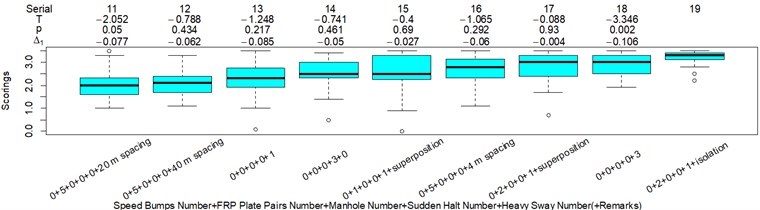
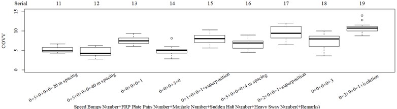
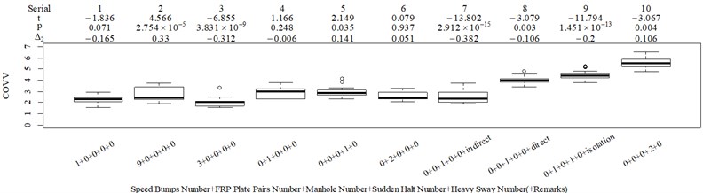
The L27(313) orthogonal test table is used to optimize the parameters in the COVV model. The parameters to be optimized and their alternative values are shown in Table 1, the initial alternative values are chosen empirically. The reason why and are added to the parameters is because different and even the same standard has varied specification for these parameters. ISO 2631-1 sets 1.4 and 1.4 for the synthetic of translational RMS while 1 and 1 for PVTV; BS 6841 sets 1 and 1 for the synthetic of translational RMS; Mansfield and Maeda [31] suggest 2.2 and 2.4. The NMSEs for RMS, MTVV, VDV, PVTV and COVV in the parameter set in Table 1 are shown in Table 2. The best parameter set for COVV in Table 2 is the 22th parameter set, the NMSE reaches the lowest value to 0.340, the parameter set is 1.2, 0.4, 0.5, 1.8, 1.5, 0.6, 0.02, 0.6, 0.8, 1.4, 14, 1.8, 1, the boxplot for the best parameter set COVV is shown in Fig. 7. Fig. 7 has the same serial number as Fig. 8, the values between the below and the neighboring right column are always lower or equal to 0 in Fig. 8. Fig. 8 includes all the designed scenarios. in Fig. 8 is defined as the difference between the mean values in the below column and the neighboring right column divided by the mean value in the neighboring right column, the subscription 1 means the values are concerned with the subjective scorings, and if the subscription is 2, it means the values are concerned with the objective evaluation indexes. is another auxiliary judging measure for the performances of the objective evaluation indexes. It describes the discrepancy between subjective scoring results and objective evaluation results. It’s ideal value is 0.
Table 1The initial alternatives for the parameters in the COVV model
Parameter | Alternatives | Parameter | Alternatives | Parameter | Alternatives |
0.8, 1, 1.2 | 0.3, 0.4, 0.5 | 0.5, 0.6, 0.7 | |||
1.6, 1.7, 1.8 | 1.5, 2, 2.5 | 0.4, 0.5, 0.6 | |||
0.01, 0.02, 0.03 | 0.5, 0.6, 0.7 | 0.8, 1, 1.4 | |||
0.8, 1, 1.4 | 12, 13, 14 | 1.5, 1.8, 2.1 | |||
1, 1.5, 2 |
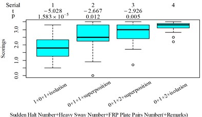
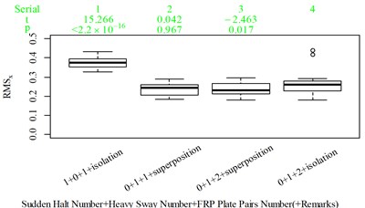
There are obviously three major problems in Fig. 7: (1) there is no significant difference between column 10 and 14 (–0.585, 0.562), which is contradictory to the results in Fig. 8 where the values in column 10 is significantly lower than the values in column 14; (2) the values in column 14 should be highly significantly higher than the values in column 11, as shown in Fig. 8, whereas the evaluation results is totally on the contrary (–3.8498, 3.388×10⁻⁴); (3) too much vibration information is integrated in scenarios represented by column 13, 15, 17, 19, especially when compared to column 18 which also includes the heavy sway excitation.
To solve the first and the second major problems in Fig. 9 at the same time, we can assign more weight to the non reference local impacts when there is more axis vibration information in the reference local impact, which means to increase the intercept item .
Table 2Fitting errors of the indexes
Index | NMSE | Index | NMSE | Index | NMSE |
RMS | 0.409 | MTVV | 0.440 | VDV | 0.415 |
PVTV | 0.548 | COVV(1) | 0.405 | COVV(2) | 0.429 |
COVV(3) | 0.393 | COVV(4) | 0.368 | COVV(5) | 0.405 |
COVV(6) | 0.473 | COVV(7) | 0.409 | COVV(8) | 0.456 |
COVV(9) | 0.460 | COVV(10) | 0.373 | COVV(11) | 0.441 |
COVV(12) | 0.428 | COVV(13) | 0.376 | COVV(14) | 0.399 |
COVV(15) | 0.407 | COVV(16) | 0.385 | COVV(17) | 0.400 |
COVV(18) | 0.506 | COVV(19) | 0.391 | COVV(20) | 0.380 |
COVV(21) | 0.452 | COVV(22) | 0.340 | COVV(23) | 0.425 |
COVV(24) | 0.431 | COVV(25) | 0.412 | COVV(26) | 0.433 |
COVV(27) | 0.418 | ||||
COVV(*) means the *th parameter set in the L27(313) orthogonal test in Table 1 | |||||
In this way, relatively more vibration information is integrated in column 14 rather than column 11 in Fig. 7 because the major vibrational axis in scenarios represented by column 14, 11 in Fig. 7 are , axis, respectively. Relatively more vibration information is integrated in column 14 rather than column 10 in Fig. 7 because the excitation numbers in scenario represented by column 14 in Fig. 7 is higher, as shown in Fig. 4(l), (m). To partly solve the third major problem in Fig. 9, we can assign more weight to the non reference local impacts when there is more y axis vibration information in the reference local impact. In this way, relatively more vibration information is integrated in column 18 rather than column 13, 15, 17, 19 in Fig. 7 because there are more major vibration durations beyond the reference local impact in scenario represented by column 18 in Fig. 7, as shown in Fig. 4(n), (o), (q), (r), (s). More consistency will also be achieved between column 13 and 15 in Fig. 7, there is no significant difference between the two columns (–0.019, 0.985), which is contradictory to the results in Fig. 8 where the values in column 13 is significantly lower than the values in column 15 (–3.055, 0.004), relatively more vibration information would be integrated to column 15 because the corresponding scenario includes one more FRP slab pair excitation. Note that we cannot assign more weight to the non reference local impacts when there is more axis vibration information in the reference local impact, because it would lead to highly contradictory results with Fig. 8 when compare column 11 and 12 in Fig. 7 to column 8-10, 14 in Fig. 7, much relatively more vibration information would be integrated to column 11 and 12 in Fig. 7. According to the above analysis, the in Eq. (12) should be replaced by in Eq. (17). In order to further solve the third major problem in Fig. 7, we can lower the , because the translational axes contribution ratios in column 13, 15, 17, 19 in Fig. 7 are 0.761, 0.747, 0.743, 0.754, respectively, suggesting too much vibration information in the axis is integrated:
where is the rectified intercept item.
Combining the analysis between Fig. 7 and 10 and range analysis results for Table 1, the alternatives in Table 1 are changed into the alternatives in Table 3. Note that the range analysis is only an auxiliary judging measurement, because it alone can result in local optimum results. When the in Eq. (12) is replaced by in Eq. (17), the NMSEs for COVV in parameter set shown in Table 3 are shown in Table 4. The best parameter set for COVV in Table 3 is the 4th parameter set, the NMSE is 0.354, the parameter set is 0.8, 0.2, 0.6, 1.6, 1.6, 0.4, 0.01, 0.6, 0.8, 0.6, 15, 2.1, 1.9, the boxplot for the best parameter set COVV is shown in Fig. 9, the column sequence in this boxplot is in accordance with that in Fig. 8.
Fig. 7Boxplot of COVV in the 22th parameter set in Table 2 for all the designed scenarios: a) the results for scenario 1-10; b) the results for scenario 11-19
a)
b)
Fig. 8Boxplot of subjective scorings for all the designed scenarios: a) the results for scenario 1-10; b) the results for scenario 11-19
a)
b)
value and value between column 10 and 14 in Fig. 9 is –0.877, 0.385, respectively, it means increasing for the sudden halt excitation is not enough, more duration rather than peak value should be stressed for this excitation type, therefore the integration order should be lowered. This is the same for the heavy sway excitation type, because the comparison between column 17 and 18 in Fig. 9 show that the ride comfort in the scenario containing 3 consecutive heavy sways is highly underestimated on condition that the vibration perception window already gives enough weight to the vibration information beyond the reference integration location, more duration rather than peak value should be stressed, the peak value comparisons for scenarios including at least a heavy sway are shown in Fig. 5(m) and (u). Note that there is no evidence in Fig. 9 to show that the current integration order for the axis has a major problem. In this case, the results suggest different integration order for different translational axes, so Eq. (15)-(17) should be rectified into Eq. (18)-(20), respectively:
where is the integration order for axis , , , .
Table 3The second batch alternatives for the parameters in the COVV model
Parameter | Alternatives | Parameter | Alternatives | Parameter | Alternatives |
0.8, 1, 1.2 | 0.1, 0.2, 0.3 | 0.5, 0.6, 0.7 | |||
1.5, 1.6, 1.7 | 1.6, 1.8, 2 | 0.4, 0.5, 0.6 | |||
0.01, 0.02, 0.03 | 0.5, 0.6, 0.7 | 0.6, 0.8, 1 | |||
0.5, 0.6, 0.7 | 13, 14, 15 | 1.5, 1.8, 2.1 | |||
1.5, 1.7, 1.9 |
Table 4Fitting errors for the second batch COVV parameter configurations
Index | NMSE | Index | NMSE | Index | NMSE |
COVV(1) | 0.406 | COVV(2) | 0.381 | COVV(3) | 0.387 |
COVV(4) | 0.354 | COVV(5) | 0.375 | COVV(6) | 0.385 |
COVV(7) | 0.382 | COVV(8) | 0.389 | COVV(9) | 0.409 |
COVV(10) | 0.366 | COVV(11) | 0.370 | COVV(12) | 0.398 |
COVV(13) | 0.389 | COVV(14) | 0.393 | COVV(15) | 0.397 |
COVV(16) | 0.368 | COVV(17) | 0.364 | COVV(18) | 0.408 |
COVV(19) | 0.369 | COVV(20) | 0.379 | COVV(21) | 0.400 |
COVV(22) | 0.361 | COVV(23) | 0.369 | COVV(24) | 0.397 |
COVV(25) | 0.374 | COVV(26) | 0.390 | COVV(27) | 0.400 |
COVV(*) means the * th parameter set in the L27(313) orthogonal test in Table 3 | |||||
The rotational axis contribution ratios in column 13, 15, 17, 19 in Fig. 9 are 0.532, 0.491, 0.473, 0.478, respectively, they are too high and are contradictory to the suggestion in ISO 2631-1, BS 6841, and many other ride comfort evaluation indexes in that the major contribution should come from the translational axes. If the integrated vibration information in the rotational axes should remains the same, then Fig. 9 suggest a even lower to satisfy consistency, then the contribution proportion in the rotational axis would be even higher. The rotational axis contribution ratios in column 7, 8 in Fig. 9 are 0.408, 0.236, respectively, and as is discussed before, these two columns especially need to integrate vibration information in the rotational axes. So the above results suggest vibration information integration in the rotational axis should be suppressed only when their values are high. In this case, a suppression order is introduced, and Eq. (19) should be replaced by Eq. (21):
where is the suppression order for axis , 1, which means there is no suppression for the translational axes, , is the suppression order in the rotational axes, 0 1.
Fig. 9Boxplot of COVV in the 4th parameter set in Table 4 for all the designed scenarios: a) the results for scenario 1-10; b) the results for scenario 11-19
a)
b)
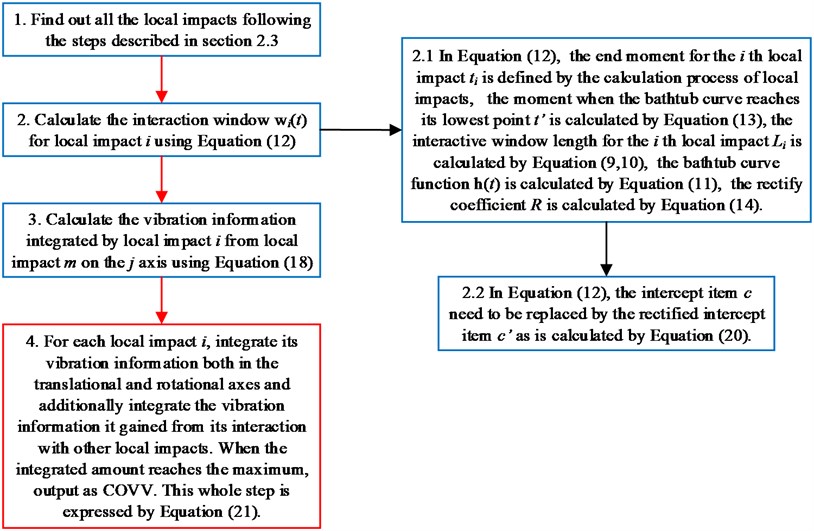
The final flowchart for the calculation of COVV is shown in Fig. 10, which is derived from the calculation processes as shown in section 2.3 and 2.4. The red arrows display the path of the main flow, the black arrows display the path of the subflow, the red frame display the final step and final output.
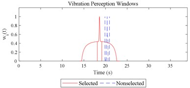
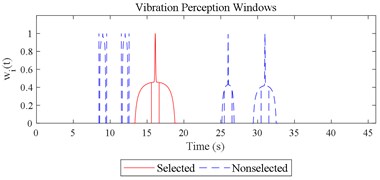
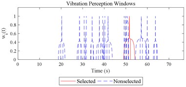
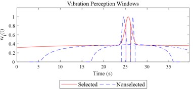
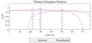
The scenario as shown in Fig. 3(l) is taken as an example for the calculation of COVV under the flowchart given by Fig. 10. The 25th parameter set in the L64(421) orthogonal test in Table 5 is adopted because it is the best parameter set for the final rectified COVV model. When step 1 and 2 in Fig. 10 is finished, the locations and the corresponding interaction windows of the calculated a total of 2 local impacts are shown in Fig. 12(l). The end moments , are 23.395 s, 63.095 s, respectively. The moments when the bathtub curve as is expressed in Eq. (11) reaches its lowest point for the 1, 2th local impact are both 0.509. The translational axes energy , are 13.616 m2 s-3, 12.640 m2 s-3, respectively. The influence energy , are 30.339 m2 s-3, 28.202 m2 s-3, respectively. The window length , are 215.707 s, 189.824 s, respectively. The rectify coefficient for the 1, 2th local impact are both 0.0018. As such, the is fixed. For Eq. (18) in step 3, the , can be calculated by using the non-weighted accelerations in the , , and axis and non-weighted rotational angular velocities in the , , and axis in moment as are calculated by Eq. (1) and using a Hilbert-Huang Transform (HHT) to calculate the frequency weighted ones [44]. When 1, they are 2.195, 0.114, 0.294, 0.005, 0.058, 0.004, respectively. When 2 they are 2.078, 0.130, 0.274, 0.008, 0.054, 0.001, respectively. With this calculation, the rectified intercept item for the 1, 2th local impact can be easily defined according to Eq. (20) and they are 1.051, 1.053, respectively. In step 3 in Fig. 10, the vibration information integrated by local impact from local impact on the axis can be defined with the already calculated and . When 1, 2, , 1.943; when 2, 1, , 1.854; the results for other combinations of , , are not shown here for simplification purposes. Finally, according to Eq. (21), the maximum vibration information is integrated when 1, as is visualized by the red mark in Fig. 12(l), the COVV is calculated as 5.171 with the aforementioned calculation results and the 25th parameter set in the L64(421) orthogonal test in Table 5.
Fig. 10Final flowchart for the calculation of COVV
3. Results for the final rectified COVV model
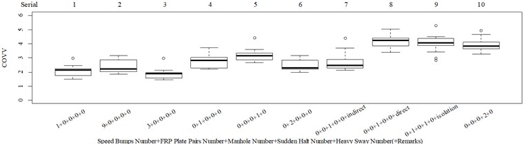
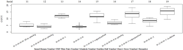
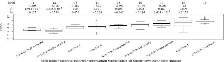
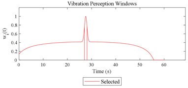
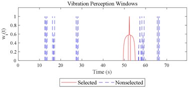
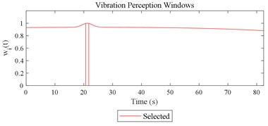
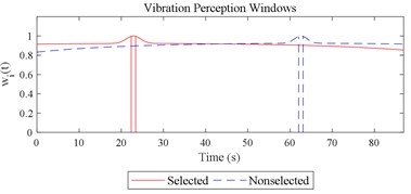
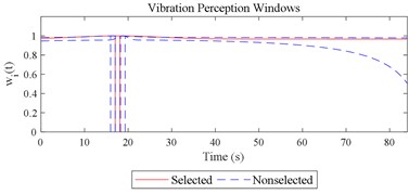
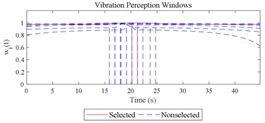
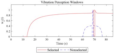
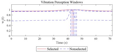
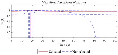
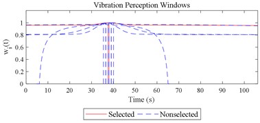
Given the revision in section 2.4, the comparing results between Fig. 8 and 9, the range analysis in Table 4, the final spreadsheet come to Table 5 and the results are shown in Table 6. Note that the orthogonal test changes from L27(313) to L64(421) because more parameters are involved. The best parameter set for COVV in Table 6 is the 25th parameter set, the NMSE is 0.325, the parameter set is 1.05, 0.14, 0.55, 1.75, 1.45, 0.25, 0.008, 0.45, 0.8, 0.36, 13.2, 1.5, 1.8, 0.625, 0.82, 1.4, 1.6. The boxplot for the 25th parameter set COVV in Table 6 is shown in Fig. 11, the column sequence in the boxplot is the same as Fig. 8. The range of between the results in Fig. 8 and 11 is [0.004, 0.448], on average is 0.118. The visualizations for the interactions between the local impacts in all the designed scenarios when parameter set for COVV is the 25th in Table 6 are shown in Fig. 12. The width between the two vertical lines in the central area of a vibration perception window in Fig. 12 is the local integration time .
Fig. 11Boxplot of COVV in the 25th parameter set in Table 6 for all the designed scenarios: a) the results for scenario 1-10; b) the results for scenario 11-19
a)
b)
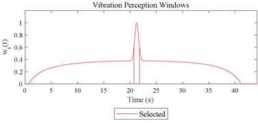
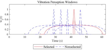
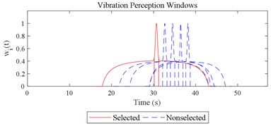
Fig. 12Visualizations for the interactions between the local impacts in all the designed scenarios when parameter set for COVV is the 25th in Table 6: a)-s) correspond to Fig. 4(a-s), respectively
a)
b)
c)
d)

e)
f)
g)
h)
i)
j)
k)
l)
m)
n)
o)
p)
q)
r)
s)
Table 5The final batch alternatives for the parameters in the COVV model
Parameter | Alternatives | Parameter | Alternatives |
1, 1.05, 1.1, 1.15 | 0.1, 0.12, 0.14, 0.16 | ||
0.4, 0.45, 0.5, 0.55 | 1.75, 1.8, 1.85, 1.9 | ||
1.4, 1.45, 1.5, 1.55 | 0.25, 0.3, 0.35, 0.4 | ||
0.0075, 0.008, 0.0085, 0.009 | 0.25, 0.3, 0.35, 0.4 | ||
0.65, 0.7, 0.75, 0.8 | 0.32, 0.34, 0.36, 0.38 | ||
12.3, 12.6, 12.9, 13.2 | 1.5, 1.6, 1.7, 1.8 | ||
1.7, 1.8, 1.9, 2 | 0.690, 0.667, 0.645, 0.625 | ||
0.78, 0.8, 0.82, 0.84 | 1.37, 1.4, 1.43, 1.48 | ||
1.6, 1.65, 1.7, 1.75 |
Table 6Fitting errors for the final batch COVV parameter configurations
Index | NMSE | Index | NMSE | Index | NMSE | Index | NMSE |
COVV(1) | 0.354 | COVV(2) | 0.369 | COVV(3) | 0.356 | COVV(4) | 0.356 |
COVV(5) | 0.347 | COVV(6) | 0.350 | COVV(7) | 0.348 | COVV(8) | 0.376 |
COVV(9) | 0.336 | COVV(10) | 0.370 | COVV(11) | 0.337 | COVV(12) | 0.375 |
COVV(13) | 0.350 | COVV(14) | 0.365 | COVV(15) | 0.334 | COVV(16) | 0.389 |
COVV(17) | 0.388 | COVV(18) | 0.360 | COVV(19) | 0.350 | COVV(20) | 0.343 |
COVV(21) | 0.337 | COVV(22) | 0.329 | COVV(23) | 0.354 | COVV(24) | 0.333 |
COVV(25) | 0.325 | COVV(26) | 0.349 | COVV(27) | 0.358 | COVV(28) | 0.368 |
COVV(29) | 0.338 | COVV(30) | 0.355 | COVV(31) | 0.347 | COVV(32) | 0.348 |
COVV(33) | 0.378 | COVV(34) | 0.348 | COVV(35) | 0.341 | COVV(36) | 0.348 |
COVV(37) | 0.337 | COVV(38) | 0.340 | COVV(39) | 0.361 | COVV(40) | 0.327 |
COVV(41) | 0.383 | COVV(42) | 0.391 | COVV(43) | 0.361 | COVV(44) | 0.387 |
COVV(45) | 0.330 | COVV(46) | 0.368 | COVV(47) | 0.350 | COVV(48) | 0.393 |
COVV(49) | 0.353 | COVV(50) | 0.346 | COVV(51) | 0.332 | COVV(52) | 0.357 |
COVV(53) | 0.345 | COVV(54) | 0.354 | COVV(55) | 0.355 | COVV(56) | 0.367 |
COVV(57) | 0.353 | COVV(58) | 0.372 | COVV(59) | 0.353 | COVV(60) | 0.339 |
COVV(61) | 0.352 | COVV(62) | 0.349 | COVV(63) | 0.330 | COVV(64) | 0.357 |
COVV(*) means the * th parameter set in the L64(421) orthogonal test in Table 5 | |||||||
4. Discussion
Fig. 11 is generally in consistent with Fig. 8, which indicate the 25th parameter set COVV in Table 6 has good performances. The NMSE for the 25th parameter set COVV in Table 6 is 0.325 and is 20.538 % lower than that of RMS which is the best evaluation index given by ISO 2631-1 for the designed scenarios. PVTV performs worst among the reference indexes, its NMSE is 68.615 % higher than that of the 25th parameter set COVV in Table 6 and 33.985 % higher than that of RMS. VDV, MTVV respectively give only1.467 %, 7.579 % higher NMSE than RMS, and according to their varied performances, they cannot completely replace or be replaced by RMS.
The range and average between Fig. 8 and 11 is also generally acceptable. between Fig. 8 and 11 reaches its highest level of 0.448 between column 2 and 3, but it is hard to adjust because if the is lowered to ensure less vibration information integration in column 2, then vibration information integration in column 12 would be not enough, as shown in Fig. 12(c) and (f). The between column 2 and 3 in Fig. 5(b), (d) are 0.485, 0.506, respectively, which indicate RMS and VDV performs even worse when compared to the 25th parameter set COVV in Table 6 in scenarios represented by these two columns. But 0.448 is still too high and suggest the method to define be further optimized in future research. Nevertheless, this is still able to show that there is no significant difference between column 1 and 2 in Fig. 11, the is only 0.104, which is not the case for RMS, VDV, and PVTV, the between column 1 and 2 in Fig. 5(b), (d), (e) are 0.356, 0.346, 0.254, respectively, they are too high and show that both RMS, VDV, and PVTV can give highly significantly contradictory results between the scenarios represented by Fig. 4(a) and (c). In Fig. 11, the values in column 16 is highly significantly higher than the values in column 11 and 12, which shows the 25th parameter set COVV in Table 6 gives consistent evaluation results with the results in Fig. 8, whereas this is not the case for RMS, VDV, and PVTV, as shown in column 8-10 in Fig. 5(b), (d), (e), the values between these columns are not significantly different or not highly significantly different. In this case, adding a normal distribution density curve to characterize the vibration perception window has gained its effect, as shown in Fig. 12(h). Note that the normal distribution density curve can add to the difference between column 16 and column 11 or 12 in Fig. 11 is also due to its function to avoid excessive vibration information in scenarios represented by Fig. 12(f) and (g). In Fig. 11, the values in column 7 is not significantly different to the values in column 6, which shows the 25 th parameter set COVV in Table 6 gives consistent evaluation results with the results in Fig. 8, the is only 0.052, whereas this is not the case for MTVV and VDV, as shown in column 5, 6 in Fig. 5(c), (d), the values between the two columns are highly significantly different, the reaches a high level of 0.648 and 0.959, respectively. In this case, involving rotational axis vibration information integration is obviously necessary. The 25th parameter set COVV in Table 6 also suggest the way to integrate rotational axis vibration information as shown in Eq. (21) can perform far better than the way provided by PVTV for all the designed scenarios, PVTV is a simple expansion for RMS and suffers from the difficulty in standardizing the total integration time , however, this is not the case for COVV.
None of RMS, MTVV, VDV, PVTV is able to give highly consistent evaluation results with subjective scoring results in group 3, as shown in Fig. 5(f-j). RMS, VDV, and PVTV all used all the vibration information in the entire timeline, but they all fail to express that the real ride comfort in scenario represented by column 3 in Fig. 5(f) is significantly higher then the real ride comfort in scenario represented by column 2 in Fig. 5(f). Fig. 5(i) shows the integration order 4 for VDV is too high, it overly emphasized the peak values in column 2 or highly significantly underestimated the durations in column 3, the peak values comparisons are shown in Fig. 5(h), the durations comparisons are shown in Fig. 3(k-m). Fig. 5(g) shows the integration order 2 for RMS is still too high, because the values in column 2 are significantly higher than the values in column 3, this is on condition that the total integration time in scenarios represented by Fig. 3(k-m) are designed to be the same. Fig. 5(j) shows the values in column 2 is not significantly different to the values in column 3 and is contradictory to the results in Fig. 5(f) where the values in column 2 is significantly lower to the values in column 3, which also suggest the integration order for PVTV should be lowered. Fig. 5(h) shows MTVV neglected the vibration information beyond the maximum part of a local integration time , which highly significantly underestimated the durations in scenario represented by column 3. The values between column 5 and 10 in Fig. 11 are highly significantly different ( –25.161, 2.2×10⁻¹⁶), the values between column 10 and 14 in Fig. 11 are significantly different (–2.712, 0.010), which show the 25th parameter set COVV in Table 6 is able to give highly consistent evaluation results with subjective scoring results in group 3. For the 25th parameter set COVV in Table 6, the is 0.82 and is lower than 2 or 4, which is able to emphasize more of the durations rather than the peak values of the sudden halt excitation type and thus gives more consistent evaluation results accordingly; the vibration perception windows covers the 3 sudden halt excitations and assigns comparable weight to the sudden halts beyond the selected reference sudden halt, as shown in Fig. 12(m), which shows the rectified interception item has gained its effect. COVV is contradictory to MTVV in that it also integrate vibration information beyond a local integration time , which helps to integrate necessary vibration information and achieves better consistency.
5. Conclusions
The devised COVV model achieves greater consistency and accuracy than RMS, MTVV, VDV, and PVTV in evaluation of road ride comfort. Its interactive mechanism is able to express the facts: (1) highly concentration of vibration information alone can add to total discomfort; (2) the interactive strength between localized major vibrations does not change sharply in a range neither too close nor too far away, which means the total discomfort remain stable in this range; (3) not all vibrations in the entire timeline need to be integrated to express real road ride comfort, only the segment where a major vibration together with its interactions with other major vibrations reaches the maximum should be used; (4) the interactive form vary according to the characteristics of a major vibration, a major vibration can interact with a wider range of other major vibrations when its intensity is higher, a major vibration can have more interactive strength with other major vibrations if it contains more vibration information in the or axis; (5) current integration order 2 for RMS, MTVV, PVTV and 4 for VDV are too high; (6) integration order should vary among different translational axes, rotational axis integration order should be suppressed when rotational axis vibration information is high. The single road ride comfort evaluation index COVV can be apply to various actual scenarios where vibration information distribution characteristics vary among axes or spacetime.
6. Supplementary materials
All the materials, data, and protocols associated with this research are available online at http://dx.doi.org/10.17632/w5zbjpdrsw.2.
References
-
Kyung G., Nussbaum M. A., Babski Reeves K. Driver sitting comfort and discomfort: part I – use of subjective ratings in discriminating car seats and correspondence among ratings. International Journal of Industrial Ergonomics, Vol. 38, Issues 5-6, 2008, p. 516-525.
-
Griffin M. J., Erdreich J. Handbook of Human Vibration. First Edition, Academic Press, Cambridge, 2012.
-
Dupuis H., Zerlett G. The Effects of Whole-Body Vibration. 1st Edition, Springer, New York, 1986.
-
Liu J., Xu Z. D., Shao Y. M., Deng C. L., Song X. H., Jiang G. L. An optimization design method for a body mounting system of a heavy vehicle. Journal of Materials: Design and Applications, Vol. 233, Issue 7, 2019, p. 1352-1362.
-
Xin F. L., Qian L. J., Du H. P., Li W. H. Multi-objective robust optimization design for powertrain mount system of electric vehicles. Journal of Low Frequency Noise Vibration and Active Control, Vol. 36, Issue 3, 2017, p. 243-260.
-
Mastinu G., Ploechl M. Road and Off-Road Vehicle System Dynamics Handbook. 1st Edition, CRC Press, Boca Raton, 2014.
-
Zhou H., Qiu Y., Lot R., Gao J. D., Yang J. S. A vehicle-human model for analysis of ride comfort predominated with vertical and pitch motions. Proceedings of the 25th International Symposium on Dynamics of Vehicles on Roads and Tracks, Rockhampton, 2017.
-
Fuentes L., Camargo R., Martínez Arguelles G., Komba J. J., Naik B., Walubita L. F. Pavement serviceability evaluation using whole body vibration techniques: a case study for urban roads. International Journal of Pavement Engineering, 2019, https://doi.org/10.1080/10298436.2019.1672872.
-
Wang X. R. A Study on Evaluation Method of Expressway Pavement Roughness Based on Riding Comfort Theory. Master’s Thesis, Beijing University of Technology, Beijing, 2014, (in Chinese).
-
Patelli G., Morioka M., Griffin M. J. Frequency-dependence of discomfort caused by vibration and mechanical shocks. Ergonomics, Vol. 61, Issue 8, 2018, p. 1102-1115.
-
Mansfield N. J., Holmlund P., Lundström R. Comparison of subjective responses to vibration and shock with standard analysis methods and absorbed power. Journal of Sound and Vibration, Vol. 230, Issue 3, 2000, p. 477-491.
-
Dickey J. P., Eger T. R., Oliver M. L., Boileau P. E., Trick L. M., Edwards A. M. Multi-axis sinusoidal whole-body vibrations: part II – relationship between vibration total value and discomfort varies between vibration axes. Journal of Low Frequency Noise Vibration and Active Control, Vol. 26, Issue 3, 2007, p. 195-204.
-
Standard Guide for Conducting Subjective Pavement Ride Quality Ratings. American Society for Testing and Materials, West Conshohocken, 2018.
-
Nakamura V. F. Serviceability Ratings of Highway Pavements. Purdue University, Lafayette, 1962.
-
Sayers M. W., Gillespie T. D., Queiroz C. A. The International Road Roughness Experiment: Establishing Correlation and a Calibration Standard for Measurements. The World Bank, Washington DC, 1986.
-
Highway Performance Assessment Standards. Research Institute of Highway Ministry of Transport, Ministry of Transport of the People’s Republic of China, Beijing, 2018, (in Chinese).
-
Loprencipe G., Zoccali P. Ride quality due to road surface irregularities: comparison of different methods applied on a set of real road profiles. Coatings, Vol. 7, Issue 5, 2017, p. 59.
-
Papagiannakis A., Raveendran B. International standards organization-compatible index for pavement roughness. Transportation Research Record, Vol. 1643, Issue 1, 1998, p. 110-115.
-
Liu C., Herman R. Road profile, vehicle dynamics, and ride quality rating. Journal of Transportation Engineering, Vol. 125, Issue 2, 1999, p. 123-128.
-
Múčka P. Current approaches to quantify the longitudinal road roughness. International Journal of Pavement Engineering, Vol. 17, Issue 8, 2016, p. 659-679.
-
Hegmon R. R. Some Results from Ongoing Research on Road Roughness. American Society for Testing and Materials, West Conshohocken, 1992.
-
Gagarine N., Mekemson J. R., Nemmers C. J. Assessing IRI vs. PI as a Measurement of Pavement Smoothness. Missouri Department of Transportation, Jefferson City, 2006.
-
Mechanical Vibration and Shock-Evaluation of Human Exposure to Whole-Body Vibration: Part I – General Requirements. International Standard Organization, Geneva, 1997.
-
Zhao J., Wang F., Yu B., Tong P., Chen K. Experimental study on the ride comfort of a crawler power chassis scale model based on the similitude theory. Chinese Journal of Mechanical Engineering, Vol. 28, Issue 3, 2015, p. 496-503.
-
Griffin M. J. A comparison of standardized methods for predicting the hazards of whole-body vibration and repeated shocks. Journal of Sound and Vibration, Vol. 215, Issue 4, 1998, p. 883-914.
-
Griffin M. J. Discomfort from feeling vehicle vibration. Vehicle System Dynamics, Vol. 45, Issues 7-8, 2007, p. 679-698.
-
Miwa T. Evaluation methods for vibration effect: part 8 – the vibration greatness of random waves. Industrial Health, Vol. 7, Issue 3, 1969, p. 89-115.
-
Ueckermann A., Steinauer B. The weighted longitudinal profile: A new method to evaluate the longitudinal evenness of roads. Road Materials and Pavement Design, Vol. 9, Issue 2, 2008, p. 135-157.
-
Paddan G. S., Griffin M. J. Effect of seating on exposures to whole-body vibration in vehicles. Journal of Sound and Vibration, Vol. 253, Issue 1, 2002, p. 215-241.
-
Rodean S., Arghir M. Absorbed power as a method to evaluate the health risk of seated occupants exposed to vertical vibration. Special Issue: 80th Annual Meeting of the International Association of Applied Mathematics and Mechanics, Vol. 9, Issue 1, 2009, p. 145-146.
-
Mechanical Vibration and Shock-Evaluation of Human Exposure to Whole-Body Vibration: Part 5 – Method for Evaluation of Vibration Containing Multiple Shocks. International Standard Organization, Geneva, 2018.
-
Tan Y. Research on Quantitative Control of Road Surface Roughness. Master’s Thesis, Chang’an University, Xi’an, 2005, (in Chinese).
-
Mansfield N. J., Maeda S. Subjective ratings of whole-body vibration for single-and multi-axis motion. Journal of The Acoustical Society of America, Vol. 130, Issue 6, 2011, p. 3723-3728.
-
Thuong O., Griffin M. J. The vibration discomfort of standing people: Evaluation of multi-axis vibration. Ergonomics, Vol. 58, Issue 10, 2015, p. 1647-1659.
-
Guide to Measurement and Evaluation of Human Exposure to Whole-Body Mechanical Vibration and Repeated Shock. British Standards Institution, London, 1987.
-
Elmes D. G., Kantowitz B. H., Roediger III H. L. Research Methods in Psychology. 9th Edition, Cengage Learning, Boston, 2011.
-
Breiman L. Classification and Regression Trees. 1st Edition, Routledge, Abingdon, 2017.
-
Fairley T. E., Griffin M. J. The apparent mass of the seated human body: vertical vibration. Journal of Biomechanics, Vol. 22, Issue 2, 1989, p. 81-94.
-
Wasserstein R. L., Lazar N. A. The ASA’s statement on p-values: context, process, and purpose. American Statistician, Vol. 70, Issue 2, 2016, p. 129-133.
-
Alhasan A. D., White J., Brabanter K. Wavelet filter design for pavement roughness analysis. Computer-Aided Civil and Infrastructure Engineering, Vol. 31, Issue 12, 2016, p. 907-920.
-
Nguyen T., Lechner B., Wong Y. D., Tan J. Y. Bus Ride Index – a refined approach to evaluating road surface irregularities. Road Materials and Pavement Design, 2019, https://doi.org/10.1080/14680629.2019.1625806.
-
The Beibo Law is a Part of Social Psychology, https://www.google.com/amp/s/kknews.cc/other/vp38m82.amp (in Chinese).
-
Yu C. Research of Bathtub Curve and Related Model Issues. Master’s Thesis, Beihang University, Beijing, 2014, (in Chinese).
-
Huang N. E., Shen Z., Long S. R., Wu M. C., Shih H. H., Zheng Q. A., Yen N. C., Tung C. C., Liu H. H. The empirical mode decomposition and the Hilbert spectrum for nonlinear and non-stationary time series analysis. Proceedings of The Royal Society A: Mathematical, Physical and Engineering Sciences, Vol. 454, Issue 1971, 1998, p. 903-995.
About this article

This research was funded by National Natural Science Foundation of China (#71471134).
