Consideration on lateral vibration of automobiles in quasi-planar model with wheel separation and road deformation taken into account

Vu Cong, Ham; Phung Manh, Cuong; Tran Quang, Dung

doi:10.21595/jve.2020.21670

Journal of Vibroengineering

Browse Journal

Submit article

Published: 16 January 2021

Check for updates

Consideration on lateral vibration of automobiles in quasi-planar model with wheel separation and road deformation taken into account

Ham Vu Cong¹

Cuong Phung Manh²

Dung Tran Quang³

^{1, 2, 3}Faculty of Mechanics, Le Quy Don Technical University, Hanoi, Vietnam

Corresponding Author:

Cuong Phung Manh

Cite the article Download PDF

Downloads 871

Abstract

This article considers lateral vibration of an automobile in a so-called quasi-planar model where both the loss of contact and road deformation are taken into account. The automobile with dependent suspension is modeled as a vibration system which has two masses and four degrees of freedom. The deformed road is modeled as an elastic beam which has uniform rectangular cross-section, is simply supported at the two ends and lies on the Kelvin's visco-elastic ground. The loss of contact and the change in dimensions of contact areas are considered. The differential equations of motion of the vehicle-road coupled system which contains a partial differential equation are transformed into a set of all ordinary differential equations by applying the Bubnov-Galerkin’s method. A procedure for numerically solving the transformed differential equations of motion is proposed. Some illustrating results coming from numerical consideration are also presented in the paper.

Consideration on lateral vibration of automobiles in quasi-planar model with wheel separation and road deformation taken into account

Highlights

We proposed a new of vehicle vibration model which called quasi-planar.
The change in dimension of the contact area between wheel with road surface is considered.
By applying the Bubnov-Galerkin's method, we get a set of all ordinary differential equations.
Some illustrating numerical example are presented to confirm the dynamic response of vehicle with taking and not taking wheel separation.

1. Introduction

Vibration of automobiles while moving on rough roads appears naturally and frequently. Among components of vibration, the ones which cause vertical vibration of points on the automobile are more considerable. When the level of vibration exceeds a definite threshold, one or more wheels may separate from the road surface and the state of contact between the wheels and the road surface is broken. This phenomenon is called as the loss of contact, or wheel separation. The loss of contact reduces controllability of the automobile in both velocity and direction, therefore, the safety of movement. For this reason, it is needed to take the loss of contact (wheel separation) into account while considering vibration of automobiles.

Without wheel separation, the vehicle dynamics attract a lot of attention from the researchers. In [1, 2], the road damage caused by heavy commercial vehicles is investigated using a quarter-vehicle model with two degree of freedom (DOF) or a half vehicle with four DOF. Using a four DOF model, the dynamics of vehicles with nonlinear spring and damping element is considered by Zhu and Ishitobi in [3]. The researches on vehicle-track and vehicle-bridge interaction have developed rapidly, in which the vehicle and the road are linked by the tire forces. In [4], a vibration seven DOF model of heavy vehicle-road coupled system with independent suspensions is presented, where the pavement-foundation is modeled as a double-layer plate on a linear viscoelastic foundation. Using the Galerkin’s method and quick direct integral method, the dynamical behaviour of the vehicle-pavement-foundation coupled system is numerically investigated. Li et al. [5] analyzed nonlinear responses of a seven DOF vehicle moving along a simply supported double-layer rectangular plate on a nonlinear viscoelastic foundation. The effects of system parameters on vertical acceleration of vehicle body and pavement displacements are also studied.

However, wheel separation has still appeared in very few researches on dynamics of vehicle-road coupled system. Cheng et la [6] investigated the vehicle-bridge interaction taking into account the effects of separation and impact on re-establishment of contact between the moving vehicle and bridge. The dynamic response of a stationary structure made of several Timoshenko beams under moving oscillator with the separation and reattachment phenomena is studied by Baeza and Ouyang in [7]. Stăncioiu et al. [8] inspected the vibration of a continuous beam resting on elastic supports excited by a moving two-axle system with separation. The dynamic response of the system can be very different from the case of not taking separation into account. Base on linear complementary relation linking relative displacement and interaction force between the wheel and the bridge at contact points, Zhu et al. [9] established a model to consider separation in a vehicle-bridge system. The influence of velocity, the vehicle to bridge mass ratio and the road roughness on separation is studied. A two DOF quarter-car model and a simply supported Euler beam representing the bridge to analyze dynamic interaction of vehicle-bridge system with separation are used in [10]. In addition, a nonlinear multiple-spring tire is modeled to describe the contact surface of tire and road instead of a point and the form of governing equations does not change whatever the tire separates from the bridge or not.

Vibration of automobiles with wheel separation taken into account has been also considered in some different models by the own authors of this paper. The quarter-car models without and with road deformation have been considered in [11, 12]. Vehicle vibrations in half-car models can be considered in two types, longitudinal and lateral vibrations. In [13], the authors investigated the longitudinal vibration of two-axle automobiles with wheel separation, but road deformation was ignored. Vibration of two-axle automobiles in spatial (full-car) model without taking road deformation has been considered in [14].

The lateral vibration is a common component of vehicle vibration in general and has a significant effect on the passenger’s ride comfort and safety of vehicles. In fact, this component of vibration even occurs more frequently than the longitudinal one. As a continuation of our researches, this paper deals with the lateral vibration of automobiles in half-car model with road deformation and wheel separation considered. The automobile with dependent suspension is modeled as a vibration system which has two masses and four degrees of freedom, while the deformed road is modeled as an elastic beam which has uniform rectangular cross-section and is simply supported at the two ends and lies on the Kelvin's viscoelastic ground. Although movements of the masses in the physical model take place in a vertical plane, the model is still called as a quasi-planar model because the change in lengths of rectangular contact areas takes place in the direction of movement that is perpendicular to the moving plane, and so does the change in pressure distribution law. The differential equations of motion of the vehicle-road coupled system including a partial differential equation are transformed into a set of all ordinary differential equations by applying the Bubnov-Galerkin’s method. Some illustrating results obtained from a numerical example are also presented to confirm the occurrence of separation and the difference of dynamic response of vehicle with taking and not taking wheel separation.

2. Vibration model and differential equations of motion

2.1. Assumptions

The lateral vibration model of automobile with dependent suspensions is created with the following assumptions:

– Body and axle of the automobile are assumed to be absolute rigids.

– Each wheel can be represented by a spring - damper couple and behavior of all spring – damper couples in the model is linear.

– Deformed road can be modeled as an elastic beam on Kelvin’s visco-elastic ground and the middle cross-section of the beam passes through the two centers of gravity.

– Lines of action of the elastic and damping forces in the same spring – damper couple coincide and perpendicular to the nominal road surface.

– Each wheel has the width unchanged while loaded and the wheel circumference part off the contact area is still round in the process of vibration.

– The contact area between each wheel and road surface (if exists) is a rectangle whose width is unchanged and equal to the original width of the wheel.

– The road profiles at two wheel tracks and the form of pressure distribution in the contact areas can be described mathematically.

– Kinematic excitation from the road upward to each wheel is calculated with using vertical fluctuation of the center point of the contact area only (not using other points).

– Automobile moves in line with a constant velocity.

2.2. Vibration model of the mechanical system

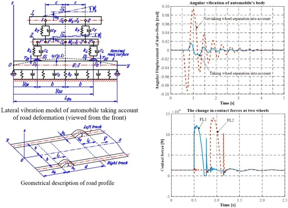
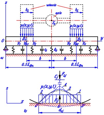
Fig. 1 shows lateral vibration model of an automobile where road deformation is taken into account. The automobile with dependent suspensions has two masses (body 1 and axle 2) whose centers of gravity are $S_{b}$ , $S_{c}$ and the inertial characteristics are ( $M_{b}$ , $J_{b}$ ), ( $M_{c}$ , $J_{c}$ ), respectively. Deformed road is modeled as an elastic beam which lies on the Kelvin's visco-elastic ground and is simply supported at the two ends.

Fig. 1Lateral vibration model of automobile taking account of road deformation (viewed from the front)

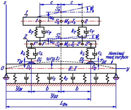
The beam with uniform rectangular cross-section has the dimensions $L_{B n}$ , $b_{B}^{x}$ and $h_{B}$ for the length, the width and the height, respectively. Material of the beam is assumed to be identical, isotropic and has the mass density $ρ$ and Young’s module $E$ . The stiffness and damping coefficient per an area unit of the ground are $k_{S}$ and $c_{S}$ , respectively.

Two suspension spring-damper couples are denoted by the notations for their stiffness and damping coefficients as ( $k_{T}$ , $c_{T}$ ). Similarly, two wheel spring-damper couples are denoted as ( $k_{L}$ , $c_{L}$ ).

The points numbered as 1, 2, 1', 2', 1", 2" are the mounting points of the spring- damper couples on the body and the axle while points $D_{1}$ and $D_{2}$ are the centers of the contact areas in cases the loss of contact does not appear.

The effect of movement on vibration of the system is expressed by the changes in height and depth of the two centers of the contact areas ( $r_{D 1}$ , $r_{D 2}$ ) and their derivatives with respect to time ( ${\dot{r}}_{D 1}$ , ${\dot{r}}_{D 2}$ ). Deformation of the road is represented by the displacement function of the beam.

Vibration of the automobile and the elastic beam are expressed in terms of the following functions of time as $u_{b} = u_{b} (t)$ , $ψ_{b} = ψ_{b} (t)$ , $u_{c} = u_{c} (t)$ , $ψ_{c} = ψ_{c} (t)$ and $w = w (y, t)$ those correspond to the displacements which are measured from the so-called natural position where both wheels still contact with the nominal road surface while all spring-damper couples in the model have no deformation.

Figure 1 also presents two typical geometrical parameters of the automobile as $b$ and $c$ , and the y-coordinates of points $D_{1}$ and $D_{2}$ .

2.3. Forces acting on the vibration system

Vertical displacements of mounting points of the spring-damper couples in the system (points numbered as 1, 2, 1', 2', 1", 2" in Fig. 1) can be determined as follows:

1

\begin{array}{l} u_{1} = u_{b} - c ψ_{b}, u_{2} = u_{b} + c ψ_{b}, \\ u_{1'} = u_{c} - c ψ_{c}, u_{2'} = u_{c} + c ψ_{c}, \\ u_{1''} = u_{c} - b ψ_{c}, u_{2^{''}} = u_{c} + b ψ_{c} . \end{array}

Fig. 2Force diagrams of body and axle of the automobile

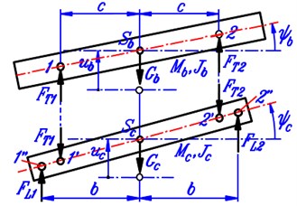
After freeing the body and the axle of automobile from the spring-damper constraints, we get their force diagrams as shown in Fig. 2.

In the diagrams, $\{G_{b}, G_{c}\}$ – forces of gravity, $\{F_{T 1}, F_{T 2}, F_{L 1}, F_{L 2}\}$ – resultant forces in four spring-damper couples, subscripts "1" and "2" imply the forces corresponding to the wheels on the left and the right side, respectively.

Resultant forces in two suspension spring-damper couples can be determined as:

2

\begin{array}{l} F_{T 1} = k_{T} (u_{1^{'}} - u_{1}) + c_{T} ({\dot{u}}_{1^{'}} - {\dot{u}}_{1}), \\ F_{T 2} = k_{T} (u_{2^{'}} - u_{2}) + c_{T} ({\dot{u}}_{2^{'}} - {\dot{u}}_{2}) . \end{array}

Vertical deformations of the wheels in case the loss of contact does not appear can be calculated as:

3

Δ z_{L 1} = w_{D 1} + r_{D 1} - u_{1^{''}}, Δ z_{L 2} = w_{D 2} + r_{D 2} - u_{2^{''}},

where $w_{D 1}$ , $w_{D 2}$ – vertical displacements of the representing beam at the center points ( $D_{1}$ , $D_{2}$ ) of the contact areas; $r_{D 1}$ , $r_{D 2}$ – the heights or depths (with respect to nominal surface of the road) of $D_{1}$ and $D_{2}$ . Basing on Fig. 1, we can determine the y-coordinates of points $D_{1}$ , $D_{2}$ and quantities $w_{D 1}$ , $w_{D 2}$ as follows:

4

\begin{array}{l} y_{D 1} = 0.5 L_{B n} - b, w_{D 1} = w (y, t) | |_{y = y_{D 1}} = w (y_{D 1}, t), \\ y_{D 2} = 0.5 L_{B n} + b, w_{D 2} = w (y, t) | |_{y = y_{D 2}} = w (y_{D 2}, t) . \end{array}

The resultant forces in the wheel spring-damper couples (equal to the contact forces) can be calculated according to the following formulas [11-14]:

5

\begin{array}{l} F_{L 1} = s_{1} [k_{L} (w_{D 1} + r_{D 1} - u_{1^{''}}) + c_{L} ({\dot{w}}_{D 1} + {\dot{r}}_{D 1} - {\dot{u}}_{1^{''}})], \\ F_{L 2} = s_{2} [k_{L} (w_{D 2} + r_{D 2} - u_{2^{''}}) + c_{L} ({\dot{w}}_{D 2} + {\dot{r}}_{D 2} - {\dot{u}}_{2^{''}})], \end{array}

where $s_{1}$ , $s_{2}$ are the contact state parameters whose values are determined by the sign of the so-called verifying values of contact forces at the two wheels:

6

\begin{array}{l} {\bar{Q}}_{1} = k_{L} (w_{D 1} + r_{D 1} - u_{1^{''}}) + c_{L} ({\dot{w}}_{D 1} + {\dot{r}}_{D 1} - {\dot{u}}_{1^{''}}), \\ {\bar{Q}}_{2} = k_{L} (w_{D 2} + r_{D 2} - u_{2^{''}}) + c_{L} ({\dot{w}}_{D 2} + {\dot{r}}_{D 2} - {\dot{u}}_{2^{''}}) . \end{array}

Particularly, the $j$ th wheel contacts the road, ${\bar{Q}}_{j} \geq$ 0 and $s_{j} =$ 1; it separates from the road if ${\bar{Q}}_{j} <$ 0 and $s_{j} =$ 0 ( $j =$ 1, 2).

2.4. Differential equations of motion of the system

2.4.1. Differential equations of motion of automobile

The equations of motion of automobile can be obtained by applying the Newton’s second law to the body and the axle of automobile using the force diagrams in Fig. 2 and relations Eqs. (2), (3), (5):

7

M_{b} {\ddot{u}}_{b} + 2 c_{T} {\dot{u}}_{b} - 2 c_{T} {\dot{u}}_{c} + 2 k_{T} u_{b} - 2 k_{T} u_{c} = - M_{b} g,

8

J_{b} {\ddot{ψ}}_{b} + 2 c_{T} c^{2} {\dot{ψ}}_{b} - 2 c_{T} c^{2} {\dot{ψ}}_{c} + 2 k_{T} c^{2} ψ_{b} - 2 k_{T} c^{2} ψ_{c} = 0,

9

\begin{array}{l} M_{c} {\ddot{u}}_{c} - 2 c_{T} {\dot{u}}_{b} + [2 c_{T} + (s_{1} + s_{2}) c_{L}] {\dot{u}}_{c} - (s_{1} - s_{2}) c_{L} b {\dot{ψ}}_{c} - s_{1} c_{L} {\dot{w}}_{D 1} - s_{2} c_{L} {\dot{w}}_{D 2} \\ - 2 k_{T} u_{b} + [2 k_{T} + (s_{1} + s_{2}) k_{L}] u_{c} - (s_{1} - s_{2}) k_{L} b ψ_{c} - s_{1} k_{L} w_{D 1} - s_{2} k_{L} w_{D 2} \\ = - M_{c} g + s_{1} (k_{L} r_{D 1} + c_{L} {\dot{r}}_{D 1}) + s_{2} (k_{L} r_{D 2} + c_{L} {\dot{r}}_{D 2}), \end{array}

10

\begin{array}{l} J_{c} {\ddot{ψ}}_{c} - 2 c_{T} c^{2} {\dot{ψ}}_{b} - (s_{1} - s_{2}) c_{L} b {\dot{u}}_{c} + [2 c_{T} c^{2} + (s_{1} + s_{2}) c_{L} b^{2}] {\dot{ψ}}_{c} + s_{1} c_{L} b {\dot{w}}_{D 1} \\ - s_{2} c_{L} b {\dot{w}}_{D 2} - 2 k_{T} c^{2} ψ_{b} - (s_{1} - s_{2}) k_{L} b u_{c} + [2 k_{T} c^{2} + (s_{1} + s_{2}) k_{L} b^{2}] ψ_{c} \\ + s_{1} k_{L} b w_{D 1} - s_{2} k_{L} b w_{D 2} = - s_{1} b (k_{L} r_{D 1} + c_{L} {\dot{r}}_{D 1}) + s_{2} b (k_{L} r_{D 2} + c_{L} {\dot{r}}_{D 2}) . \end{array}

2.4.2. Differential equation of motion of deformed road

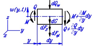
The mentioned equation can be generated by considering the equilibrium of a typical element of the beam. The force diagram of the beam element which lies at coordinate $y$ and has the axle length $d y$ is shown in Fig. 3.

Forces acting on the beam element consist of inertial force ( $d F_{q t}$ ), resultant force of Kelvin’s visco-elastic ground ( $d F_{S}$ ), force of gravity ( $d G$ ), contact force from the wheels ( $d Q_{w}$ ), the shear forces and the bending moments in the two end cross-section $\{Q, Q + (\partial Q / \partial y) d y, M, M + (\partial M / \partial y) d y\}$ .

Fig. 3a) Force diagram of a typical beam element, b) the dimension of beam cross-section

a)

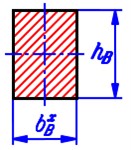
b)

The expressions of four first forces can be written as:

11

\begin{array}{l} d F_{q t} = ρ b_{B}^{x} h_{B} \frac{\partial^{2} w}{\partial t^{2}} d y, d F_{S} = (k_{S} w + c_{S} \frac{\partial w}{\partial t}) b_{B}^{x} d y, \\ d G = ρ g b_{B}^{x} h_{B} d y, d Q_{w} = \{\int_{(d_{c j})} p (x, y, t) d x\} d y, \end{array}

where $w = w (y, t)$ – displacement function of the beam, $d_{c j}$ – the length of the $j$ th contact area ( $j =$ 1, 2) in the direction of movement, $p (x, y, t)$ – function of pressure distribution on the upper surface of the beam due to the load coming from the automobile, $g$ – gravitational acceleration.

Fig. 4Description of function px,y,t on beam a) and four types of pressure distribution in x-direction (1 – constant, 2 – parabolic, 3 – cosine, 4 – cosine squared)

Description of function px,y,t on beam a) and four types of pressure distribution in x-direction (1 – constant, 2 – parabolic, 3 – cosine, 4 – cosine squared)

The function of pressure distribution $p (x, y, t)$ is defined over the whole top surface of the beam but really exists in the contact areas of the wheels (Fig. 4). Moreover, this function can be taken only based on observing the fact and using assumptions. This paper still applies the expression of $p (x, y, t)$ which is proposed in [12] and has the form:

12

p (x, y, t) = \{\begin{array}{l} P_{1} (t) U_{1} (x), y_{1} \leq y \leq y_{2}, \\ P_{2} (t) U_{2} (x), y_{3} \leq y \leq y_{4}, \\ 0, o t h e r w i s e . \end{array}

In Eq. (12), the expression of $p (x, y, t)$ is assumed unchanged in y-direction in the domain of each contact area, $P_{j} (t)$ ( $j =$ 1, 2) are unknown functions of time to be found and $U_{j} (x)$ are pre-chosen expressions to describe the change of $p (x, y, t)$ in $x$ -direction over the length $d_{c j}$ of each contact area. Hence, the expressions $U_{j} (x)$ really represent the laws of pressure distribution in the contact areas.

Four typical types of pressure distribution which can be applied in considering vibration of automobiles are proposed in [12] and graphically described in Fig. 4(b). They consist of constant (rectangular), parabolic, cosine and cosine-squared distributions. In the coordinate system $O x z$ with the origin coinciding with the center of contact area and the $x$ -axis being the direction of movement, the corresponding expression of $U_{j} (x)$ is 1, 1-4 ${(x / d_{c j})}^{2}$ , $c o s (π x / d_{c j})$ , ${c o s}^{2} (π x / d_{c j})$ .

With the expression of function $p (x, y, t)$ as taken in Eq. (12), the formula of $d Q_{w}$ in Eq. (11) becomes:

13

d Q_{w} = \{\int_{(d_{c j})} P_{j} (t) U_{j} (x) d x\} d y = P_{j} (t) I_{0}^{(j)} d y,

where:

14

I_{0}^{(j)} = \int_{(d_{c j})} U_{j} (x) d x, j = 1, 2 .

For the elements which do not lie under the contact areas, we have $d Q_{w} =$ 0 because $p (x, y, t) =$ 0.

In case wheel separation does not appear, the values of $I_{0}^{(j)}$ depend on $d_{c j}$ and can be determined by using the used type of pressure distribution. For the four types of pressure distribution mentioned above, the values of $I_{0}^{(j)}$ are $d_{c j}$ , 2 $d_{c j}$ /3, 2 $d_{c j}$ / $π$ and $d_{c j}$ /2, respectively.

The equilibrium of forces in $z$ -direction and the moment equilibrium about the center of left cross-section of the element lead to these equations:

15

\frac{\partial Q}{\partial y} d y - d F_{q t} - d F_{S} - d G - d Q_{w} = 0,

16

Q = \frac{\partial M}{\partial y} = - E I \frac{\partial^{3} w}{\partial y^{3}},

where $M = - E I \frac{\partial^{2} w}{\partial y^{2}}$ for Euler-Bernoulli’s beam theory.

Putting the expression of $Q$ from Eq. (16) into Eq. (15) and using the expressions Eq. (11) and Eq. (13) of forces then taking some needed arrangements, we obtain the differential equation of motion of the beam which represents deformed road:

17

ρ h_{B} \frac{\partial^{2} w}{\partial t^{2}} + c_{S} \frac{\partial w}{\partial t} + k_{S} w (y, t) + \frac{1}{b_{B}^{x}} E I \frac{\partial^{4} w}{\partial y^{4}} + \frac{1}{b_{B}^{x}} P_{j} (t) I_{0}^{(j)} = - ρ g h_{B} .

The differential equations of motion of the mechanical system are the combination of ordinary differential Eqs. (7-10) and partial differential Eq. (17).

2.5. Simpler cases of differential equations of motion of the system

a) If the loss of contact is ignored, we can fix $s_{1} = s_{2} =$ 1. Eqs. (7), (8) and (17) are unchanged while Eq. (9), (10) become:

18

\begin{array}{l} M_{c} {\ddot{u}}_{c} - 2 c_{T} {\dot{u}}_{b} + 2 (c_{T} + c_{L}) {\dot{u}}_{c} - c_{L} {\dot{w}}_{D 1} - c_{L} {\dot{w}}_{D 2} - 2 k_{T} u_{b} + 2 (k_{T} + k_{L}) u_{c} \\ - k_{L} w_{D 1} - k_{L} w_{D 2} = - M_{C} g + k_{L} (r_{D 1} + r_{D 2}) + c_{L} ({\dot{r}}_{D 1} + {\dot{r}}_{D 2}), \end{array}

19

\begin{array}{l} J_{c} {\ddot{ψ}}_{c} - 2 c_{T} c^{2} {\dot{ψ}}_{b} + 2 (c_{T} c^{2} + c_{L} b^{2}) {\dot{ψ}}_{c} + c_{L} b {\dot{w}}_{D 1} - c_{L} b {\dot{w}}_{D 2} - 2 k_{T} c^{2} ψ_{b} \\ + 2 (k_{T} c^{2} + k_{L} b^{2}) ψ_{c} + k_{L} b w_{D 1} - k_{L} b w_{D 2} = - k_{L} b (r_{D 1} - r_{D 2}) - c_{L} b ({\dot{r}}_{D 1} - {\dot{r}}_{D 2}) . \end{array}

b) If the deformation of road is not taken into account, we have $w (y, t) =$ 0 for every $y$ and $t$ . In this situation, it is allowed to set $k_{S} = \infty$ , $c_{S} = \infty$ and Eq. (17) becomes an identity, Eqs. (7) and (8) are unchanged while Eqs. (9) and (10) have the new forms as:

20

\begin{array}{l} M_{c} {\ddot{u}}_{c} - 2 c_{T} {\dot{u}}_{b} + [2 c_{T} + (s_{1} + s_{2}) c_{L}] {\dot{u}}_{c} - (s_{1} - s_{2}) c_{L} b {\dot{ψ}}_{c} u_{c} \\ - 2 k_{T} u_{b} + [2 k_{T} + (s_{1} + s_{2}) k_{L}] - (s_{1} - s_{2}) k_{L} b ψ_{c} \end{array}

= - M_{c} g + s_{1} (k_{L} r_{D 1} + c_{L} {\dot{r}}_{D 1}) + s_{2} (k_{L} r_{D 2} + c_{L} {\dot{r}}_{D 2}),

21

\begin{array}{l} J_{c} {\ddot{ψ}}_{c} - 2 c_{T} c^{2} {\dot{ψ}}_{b} - (s_{1} - s_{2}) c_{L} b {\dot{u}}_{c} + [2 c_{T} c^{2} + (s_{1} + s_{2}) c_{L} b^{2}] {\dot{ψ}}_{c} \\ - 2 k_{T} c^{2} ψ_{b} - (s_{1} - s_{2}) k_{L} b u_{c} + [2 k_{T} c^{2} + (s_{1} + s_{2}) k_{L} b^{2}] ψ_{c} \\ = - s_{1} b (k_{L} r_{D 1} + c_{L} {\dot{r}}_{D 1}) + s_{2} b (k_{L} r_{D 2} + c_{L} {\dot{r}}_{D 2}) . \end{array}

c) If road deformation and wheel separation are ignored, the differential equations of motion of the vehicle-road coupled system are reduced to those of only automobile with the addition of setting $s_{1} = s_{2} =$ 1. In this situation, Eqs. (7) and (8) are still unchanged while Eqs. (9) and (10) respectively becomes:

22

\begin{array}{l} M_{c} {\ddot{u}}_{c} - 2 c_{T} {\dot{u}}_{b} + 2 (c_{T} + c_{L}) {\dot{u}}_{c} - 2 k_{T} u_{b} + 2 (k_{T} + k_{L}) u_{c} \\ = - M_{c} g + k_{L} (r_{D 1} + r_{D 2}) + c_{L} ({\dot{r}}_{D 1} + {\dot{r}}_{D 2}), \end{array}

23

\begin{array}{l} J_{c} {\ddot{ψ}}_{c} - 2 c_{T} c^{2} {\dot{ψ}}_{b} + 2 (c_{T} c^{2} + c_{L} b^{2}) {\dot{ψ}}_{c} - 2 k_{T} c^{2} ψ_{b} + 2 (k_{T} c^{2} + k_{L} b^{2}) ψ_{c} \\ = - k_{L} b (r_{D 1} - r_{D 2}) - c_{L} b ({\dot{r}}_{D 1} - {\dot{r}}_{D 2}) . \end{array}

3. Solving the differential equations of motion

3.1. Transforming the differential equations of motion into ordinary differential equations

The presence of a partial differential equation does not allow to solve the original differential equations of motion of the vehicle-road coupled system until now. In order to overcome this difficulty, here the Bubnov-Galerkin’s method is applied to transform those differential equations of motion into a system of all ordinary differential equations (ODEs).

According to the Bubnov-Galerkin’s method, we need to fulfil a succession of operations as follows:

1) Approximating the displacement function of the beam $w (y, t)$ with a series of $N$ terms as:

24

w (y, t) = \sum_{l = 1}^{N} T_{l} (t) Y_{l} (y) = \sum_{l = 1}^{N} T_{l} (t) s i n \frac{(2 l - 1) π y}{L_{B n}},

where $T_{l} (t)$ are unknown functions of time to be found, $Y_{l} (y) = s i n [(2 l - 1) π y / L_{B n}]$ – shape functions satisfying boundary conditions of the beam, $w (y, t) | |_{y = 0} = w (y, t) | |_{y = L_{B n}} = 0$ .

It is important to note that the functions $Y_{l} (y)$ are linearly independent and have the property of orthogonality as:

25

\int_{0}^{L_{B n}} s i n \frac{(2 l - 1) π y}{L_{B n}} s i n \frac{(2 l' - 1) π y}{L_{B n}} d y = \{\begin{array}{l} 0, l \neq l^{'}, \\ L_{B n} / 2, l = l^{'} . \end{array}

The approximation of function $w (y, t)$ as in Eq. (24) allows to define the vector of generalized coordinates:

26

\vec{q} = {[u_{b} (t), ψ_{b} (t), u_{c} (t), ψ_{c} (t), T_{1} (t), T_{2} (t), \dots, T_{N} (t)]}^{T} .

2) Putting the Eq. (24) of $w (y, t)$ into Eq. (17) leads to the following equation:

27

\begin{array}{l} ρ h_{B} \sum_{l = 1}^{N} {\ddot{T}}_{l} (t) s i n \frac{(2 l - 1) π y}{L_{B n}} + c_{S} \sum_{l = 1}^{N} {\dot{T}}_{l} (t) s i n \frac{(2 l - 1) π y}{L_{B n}} + k_{S} \sum_{l = 1}^{N} T_{l} (t) s i n \frac{(2 l - 1) π y}{L_{B n}} \\ + \frac{1}{b_{B}^{x}} E I \sum_{l = 1}^{N} \frac{(2 l - 1)^{4} π^{4}}{L_{B n}^{4}} T_{l} (t) s i n \frac{(2 l - 1) π y}{L_{B n}} + \frac{1}{b_{B}^{x}} P_{j} (t) I_{0}^{(j)} = - ρ g h_{B} . \end{array}

3) Assigning to variable $k$ consecutively the values of the set {1, 2, ..., $N$ }. With each value, multiplying Eq. (27) by $s i n [(2 k - 1) π y / L_{B n}]$ then taking the integration of the two sides with respect to variable $y$ from 0 to $L_{B n}$ (over the length of the beam), noting the orthogonality Eqs. (25), we obtain a system of $N$ ODEs as follows:

28

\begin{array}{l} ρ h_{B} \frac{L_{B n}}{2} {\ddot{T}}_{k} (t) + c_{S} \frac{L_{B n}}{2} {\dot{T}}_{k} (t) + k_{S} \frac{L_{B n}}{2} T_{k} (t) + \frac{1}{b_{B}^{x}} E I \frac{L_{B n}}{2} \frac{(2 k - 1)^{4} π^{4}}{L_{B n}^{4}} T_{k} (t) \\ + \frac{1}{b_{B}^{x}} \int_{0}^{L_{B n}} P_{j} (t) I_{0}^{(j)} s i n \frac{(2 k - 1) π y}{L_{B n}} d y = - \frac{2 ρ g h_{B} L_{B n}}{(2 k - 1) π}, k = 1, 2, . . ., N . \end{array}

In order to calculate the integration in Eq. (28), it is important to see the form Eq. (12) of function $p (x, y, t)$ and its description in Fig. 4(a). The values of $y_{1}$ , $y_{2}$ , $y_{3}$ , $y_{4}$ can be expressed in terms of the $y$ -coordinates of points $D_{1}$ , $D_{2}$ (centers of contact areas) and the width of the wheels as follows: $y_{1} = y_{D 1} - 0,5 b_{L}$ , $y_{2} = y_{D 1} + 0,5 b_{L}$ , $y_{3} = y_{D 2} - 0,5 b_{L}$ , $y_{4} = y_{D 2} + 0,5 b_{L}$

29

\Rightarrow \begin{array}{l} y_{2} + y_{1} = 2 y_{D 1}, y_{4} + y_{3} = 2 y_{D 2}, \\ y_{2} - y_{1} = y_{4} - y_{3} = b_{L} . \end{array}

The relations in Eq. (29) allow to calculate the integration in Eq. (28) as follow:

30

\int_{0}^{L_{B n}} P_{j} (t) I_{0}^{(j)} s i n \frac{(2 k - 1) π y}{L_{B n}} d y = \int_{y_{1}}^{y_{2}} P_{1} (t) I_{0}^{(1)} s i n \frac{(2 k - 1) π y}{L_{B n}} d y

+ \int_{y_{3}}^{y_{4}} P_{2} (t) I_{0}^{(2)} s i n \frac{(2 k - 1) π y}{L_{B n}} d y = \frac{2 L_{B n}}{(2 k - 1) π} s i n \frac{(2 k - 1) π b_{L}}{2 L_{B n}}

\times [P_{1} (t) I_{0}^{(1)} s i n \frac{(2 k - 1) π y_{D 1}}{L_{B n}} + P_{2} (t) I_{0}^{(2)} s i n \frac{(2 k - 1) π y_{D 2}}{L_{B n}}]

= \frac{1}{2} L_{B n} b_{B}^{x} [β_{k}^{(1)} P_{1} (t) + β_{k}^{(2)} P_{2} (t)],

where:

31

\begin{array}{l} β_{k}^{(1)} = \frac{4 I_{0}^{(1)}}{(2 k - 1) π b_{B}^{x}} s i n \frac{(2 k - 1) π b_{L}}{2 L_{B n}} s i n \frac{(2 k - 1) π y_{D 1}}{L_{B n}}, \\ β_{k}^{(2)} = \frac{4 I_{0}^{(2)}}{(2 k - 1) π b_{B}^{x}} s i n \frac{(2 k - 1) π b_{L}}{2 L_{B n}} s i n \frac{(2 k - 1) π y_{D 2}}{L_{B n}} . \end{array}

Substituting the results in Eq. (30) into Eq. (28) leads to the following equation:

32

ρ h_{B} {\ddot{T}}_{k} (t) + c_{S} {\dot{T}}_{k} (t) + [k_{S} + \frac{E I}{b_{B}^{x}} \frac{(2 k - 1)^{4} π^{4}}{L_{B n}^{4}}] T_{k} (t) + β_{k}^{(1)} P_{1} (t) + β_{k}^{(2)} P_{2} (t) = - \frac{4 ρ g h_{B}}{(2 k - 1) π}, k = 1, 2, . . ., N .

4) Expressing functions $P_{1} (t)$ , $P_{2} (t)$ and Eq. (32) in terms of generalized coordinates.

This operation is needed because functions $P_{1} (t)$ and $P_{2} (t)$ are generated in the process of transforming the partial differential Eq. (17) into ODEs. To reach the purpose, we consider the equilibrium of the forces acting on the $j$ -th wheel ( $j =$ 1, 2) in vertical direction (see Fig. 4(b)):

33

F_{L j} = R_{j},

where $R_{j}$ – reaction force from road and $F_{L j}$ – resultant force in the $j$ -th wheel spring-damper couple.

The reaction force $R_{j}$ can be calculated based on the pre-chosen pressure distribution function as:

R_{j} = \int_{- 0,5 d_{c j}}^{0,5 d_{c j}} p_{j} (x, t) b_{L} d x = b_{L} \int_{- 0,5 d_{c j}}^{0,5 d_{c j}} P_{j} (t) U_{j} (x) d x,

or:

34

R_{1} = P_{1} (t) b_{L} I_{0}^{(1)}, R_{2} = P_{2} (t) b_{L} I_{0}^{(2)} .

In order to find the expressions of forces $F_{L j}$ , we firstly use Eq. (24) to calculate $w_{D 1}$ , $w_{D 2}$ , ${\dot{w}}_{D 1}$ , ${\dot{w}}_{D 2}$ as:

35

w_{D 1} = \sum_{l = 1}^{N} T_{l} (t) s i n \frac{(2 l - 1) π y_{D 1}}{L_{B n}} = \sum_{l = 1}^{N} χ_{l}^{(1)} T_{l} (t),

w_{D 2} = \sum_{l = 1}^{N} T_{l} (t) s i n \frac{(2 l - 1) π y_{D 2}}{L_{B n}} = \sum_{l = 1}^{N} χ_{l}^{(2)} T_{l} (t),

{\dot{w}}_{D 1} = \sum_{l = 1}^{N} {\dot{T}}_{l} (t) s i n \frac{(2 l - 1) π y_{D 1}}{L_{B n}} = \sum_{l = 1}^{N} χ_{l}^{(1)} {\dot{T}}_{l} (t),

{\dot{w}}_{D 2} = \sum_{l = 1}^{N} {\dot{T}}_{l} (t) s i n \frac{(2 l - 1) π y_{D 2}}{L_{B n}} = \sum_{l = 1}^{N} χ_{l}^{(2)} {\dot{T}}_{l} (t),

where:

36

χ_{l}^{(1)} = s i n \frac{(2 l - 1) π y_{D 1}}{L_{B n}}, χ_{l}^{(2)} = s i n \frac{(2 l - 1) π y_{D 2}}{L_{B n}} .

Eqs. (5) and (35) allow to get the expressions of $F_{L j}$ :

37

\begin{array}{l} F_{L 1} = s_{1} [k_{L} (\sum_{l = 1}^{N} χ_{l}^{(1)} T_{l} (t) + r_{D 1} - u_{c} + b ψ_{c}) + c_{L} (\sum_{l = 1}^{N} χ_{l}^{(1)} {\dot{T}}_{l} (t) + {\dot{r}}_{D 1} - {\dot{u}}_{c} + b {\dot{ψ}}_{c})], \\ F_{L 2} = s_{2} [k_{L} (\sum_{l = 1}^{N} χ_{l}^{(2)} T_{l} (t) + r_{D 2} - u_{c} - b ψ_{c}) + c_{L} (\sum_{l = 1}^{N} χ_{l}^{(2)} {\dot{T}}_{l} (t) + {\dot{r}}_{D 2} - {\dot{u}}_{c} - b {\dot{ψ}}_{c})] . \end{array}

Using Eqs. (33), (34), (37) we obtain:

38

\begin{array}{l} P_{1} (t) = \frac{s_{1}}{I_{0}^{(1)} b_{L}} [k_{L} (\sum_{l = 1}^{N} χ_{l}^{(1)} T_{l} (t) + r_{D 1} - u_{c} + b ψ_{c}) \\ + c_{L} (\sum_{l = 1}^{N} χ_{l}^{(1)} {\dot{T}}_{l} (t) + {\dot{r}}_{D 1} - {\dot{u}}_{c} + b {\dot{ψ}}_{c})], \\ P_{2} (t) = \frac{s_{2}}{I_{0}^{(2)} b_{L}} [k_{L} (\sum_{l = 1}^{N} χ_{l}^{(2)} T_{l} (t) + r_{D 2} - u_{c} - b ψ_{c}) \end{array}

+ c_{L} (\sum_{l = 1}^{N} χ_{l}^{(2)} {\dot{T}}_{l} (t) + {\dot{r}}_{D 2} - {\dot{u}}_{c} - b {\dot{ψ}}_{c})] .

Putting the expressions of $P_{1} (t)$ and $P_{2} (t)$ from Eq. (38) into Eq. (32) and taking some needed arrangements lead to the following equation:

39

ρ h_{B} {\ddot{T}}_{k} (t) - (μ_{k}^{(1)} + μ_{k}^{(2)}) c_{L} {\dot{u}}_{c} + (μ_{k}^{(1)} - μ_{k}^{(2)}) c_{L} b {\dot{ψ}}_{c}

+ \sum_{l = 1}^{N} [δ_{k l} c_{S} + (μ_{k}^{(1)} χ_{l}^{(1)} + μ_{k}^{(2)} χ_{l}^{(2)}) c_{L}] {\dot{T}}_{l} (t) - (μ_{k}^{(1)} + μ_{k}^{(2)}) k_{L} u_{c}

+ (μ_{k}^{(1)} - μ_{k}^{(2)}) k_{L} b ψ_{c} + \sum_{l = 1}^{N} [δ_{k l} H_{k} + (μ_{k}^{(1)} χ_{l}^{(1)} + μ_{k}^{(2)} χ_{l}^{(2)}) k_{L}] T_{l} (t)

= - \frac{4 ρ g h_{B}}{(2 k - 1) π} - μ_{k}^{(1)} (k_{L} r_{D 1} + c_{L} {\dot{r}}_{D 1}) - μ_{k}^{(2)} (k_{L} r_{D 2} + c_{L} {\dot{r}}_{D 2}), k = 1, 2, . . ., N,

where:

40

H_{k} = k_{S} + \frac{E I}{b_{B}^{x}} \frac{(2 k - 1)^{4} π^{4}}{L_{B n}^{4}}, μ_{k}^{(1)} = \frac{s_{1} β_{k}^{(1)}}{I_{0}^{(1)} b_{L}}, μ_{k}^{(2)} = \frac{s_{2} β_{k}^{(2)}}{I_{0}^{(2)} b_{L}},

and $δ_{k l}$ – the Kronecker’s operator defined as $δ_{k l} =$ 1 if $k = l$ , and $δ_{k l} =$ 0 if $k \neq l$ .

5) Expressing Eqs. (9) and (10) in terms of the generalized coordinates. This purpose can be reached by putting the expressions of functions $w_{D 1}$ , $w_{D 2}$ , ${\dot{w}}_{D 1}$ , ${\dot{w}}_{D 2}$ from Eq. (35) into Eqs. (9), (10) as follows:

41

\begin{array}{l} M_{c} {\ddot{u}}_{c} - 2 c_{T} {\dot{u}}_{b} + [2 c_{T} + (s_{1} + s_{2}) c_{L}] {\dot{u}}_{c} - (s_{1} - s_{2}) c_{L} b {\dot{ψ}}_{c} - \sum_{l = 1}^{N} (s_{1} χ_{l}^{(1)} + s_{2} χ_{l}^{(2)}) c_{L} {\dot{T}}_{l} (t) \\ - 2 k_{T} u_{b} + [2 k_{T} + (s_{1} + s_{2}) k_{L}] u_{c} - (s_{1} - s_{2}) k_{L} b ψ_{c} - \sum_{l = 1}^{N} (s_{1} χ_{l}^{(1)} + s_{2} χ_{l}^{(2)}) k_{L} T_{l} (t) \\ = - M_{c} g + s_{1} (k_{L} r_{D 1} + c_{L} {\dot{r}}_{D 1}) + s_{2} (k_{L} r_{D 2} + c_{L} {\dot{r}}_{D 2}), \end{array}

42

J_{c} {\ddot{ψ}}_{c} - 2 c_{T} c^{2} {\dot{ψ}}_{b} - (s_{1} - s_{2}) c_{L} b {\dot{u}}_{c} + [2 c_{T} c^{2} + (s_{1} + s_{2}) c_{L} b^{2}] {\dot{ψ}}_{c}

+ \sum_{l = 1}^{N} (s_{1} χ_{l}^{(1)} - s_{2} χ_{l}^{(2)}) c_{L} b {\dot{T}}_{l} (t) - 2 k_{T} c^{2} ψ_{b} - (s_{1} - s_{2}) k_{L} b u_{c}

+ [2 k_{T} c^{2} + (s_{1} + s_{2}) k_{L} b^{2}] ψ_{c} + \sum_{l = 1}^{N} (s_{1} χ_{l}^{(1)} - s_{2} χ_{l}^{(2)}) k_{L} b T_{l} (t)

= - s_{1} b (k_{L} r_{D 1} + c_{L} {\dot{r}}_{D 1}) + s_{2} b (k_{L} r_{D 2} + c_{L} {\dot{r}}_{D 2}) .

Now the original differential equations of motion of the mechanical system have been transformed into a system of all ordinary differential Eqs. (7), (8), (41), (42) and (39). These equations can be called as the transformed differential equations of motion (TDEM). The TDEM can be solved numerically because each from them has been expressed in terms of the generalized coordinates.

3.2. Matrix form of TDEM

The TDEM can be written in matrix form as:

43

[M] \ddot{\vec{q}} + [C] \dot{\vec{q}} + [K] \vec{q} = \vec{F},

where $\vec{q}$ – vector of generalized coordinates of the form Eq. (26), $\vec{F}$ – excitation vector; [ $M$ ], [ $C$ ], [ $K$ ] – mass, damping and stiffness matrices, respectively. The two vectors have the size as $(4 + N) \times 1$ while the matrices are all square of order $(4 + N)$ .

The excitation vector has the form as:

44

\vec{F} = {[F_{1}, F_{2}, F_{3}, F_{4}, F_{5}, F_{6}, \dots, F_{4 + N}]}^{T},

where:

45

\begin{array}{l} F_{1} = - M_{b} g, F_{2} = 0, F_{3} = - M_{c} g + s_{1} (k_{L} r_{D 1} + c_{L} {\dot{r}}_{D 1}) + s_{2} (k_{L} r_{D 2} + c_{L} {\dot{r}}_{D 2}), \\ F_{4} = - s_{1} b (k_{L} r_{D 1} + c_{L} {\dot{r}}_{D 1}) + s_{2} b (k_{L} r_{D 2} + c_{L} {\dot{r}}_{D 2}), \\ F_{4 + k} = - \frac{4 ρ g h_{B}}{(2 k - 1) π} - μ_{k}^{(1)} (k_{L} r_{D 1} + c_{L} {\dot{r}}_{D 1}) - μ_{k}^{(2)} (k_{L} r_{D 2} + c_{L} {\dot{r}}_{D 2}), k = 1, 2, . . ., N . \end{array}

The mass matrix [ $M$ ] has the diagonal form as:

46

[M] = d i a g (M_{b}, J_{b}, M_{c}, J_{c}, ρ h_{B}, ρ h_{B}, \dots, ρ h_{B}) .

The stiffness matrix [ $K$ ] contains ( $4 + N$ ) rows, each of which has ( $4 + N$ ) elements and can be successively written as follows:

47

\{K_{1}\} = \{2 k_{T}, 0, - 2 k_{T}, 0, [0,0, 0, \dots, 0]\}, \{K_{2}\} = \{0,2 k_{T c}^{2,0}, - 2 k_{T c}^{2}, [0,0, 0, \dots, 0]\},

{K_{3}} = {- 2 k_{T}, 0,2 k_{T} + (s_{1} + s_{2}) k_{L}, - (s_{1} - s_{2}) k_{L} b, [- (s_{1} χ_{1}^{(1)} + s_{2} χ_{1}^{(2)}) k_{L},

- (s_{1} χ_{2}^{(1)} + s_{2} χ_{2}^{(2)}) k_{L}, \dots, - (s_{1} χ_{N}^{(1)} + s_{2} χ_{N}^{(2)}) k_{L}]},

{K_{4}} = {0, - 2 k_{T} c^{2}, - (s_{1} - s_{2}) k_{L} b, 2 k_{T} c^{2} + (s_{1} + s_{2}) k_{L} b^{2}, (s_{1} χ_{1}^{(1)} - s_{2} χ_{1}^{(2)}) k_{L} b,

(s_{1} χ_{2}^{(1)} - s_{2} χ_{2}^{(2)}) k_{L} b, \dots, (s_{1} χ_{N}^{(1)} - s_{2} χ_{N}^{(2)}) k_{L} b]},

{K_{4 + k}} = {0,0, - (μ_{k}^{(1)} + μ_{k}^{(2)}) k_{L}, (μ_{k}^{(1)} - μ_{k}^{(2)}) k_{L} b, [δ_{k 1} H_{k} + (μ_{k}^{(1)} χ_{1}^{(1)} + μ_{k}^{(2)} χ_{1}^{(2)}) k_{L},

δ_{k 2} H_{k} + (μ_{k}^{(1)} χ_{2}^{(1)} + μ_{k}^{(2)} χ_{2}^{(2)}) k_{L}, \dots, δ_{k N} H_{k} + (μ_{k}^{(1)} χ_{N}^{(1)} + μ_{k}^{(2)} χ_{N}^{(2)}) k_{L}]},

k = 1,2, \dots, N .

The damping matrix [ $C$ ] has the form similar to that of the stiffness matrix [ $K$ ] so we can obtain matrix [ $C$ ] from matrix [ $K$ ] by substituting the notations $\{H_{k}, k_{T}, k_{L}\}$ with these ones $\{c_{S}, c_{T}, c_{L}\}$ , respectively.

3.3. Initial conditions

In almost problems on vibration of automobiles moving on horizontal roads, the initial conditions commonly relate to the fact that the vehicle is running on a definitely even road surface then entering an uneven one. In this situation, theoretically, there is no vibration occurring until the initial point of time, so the values of generalized coordinates, velocities, accelerations and all quantities concerned can be determined from the static state where the automobile lies on a horizontal road with even surface. Therefore, the initial conditions for this situation can be written as follows:

48

\ddot{\vec{q}} | |_{t = 0} = 0, \dot{\vec{q}} | |_{t = 0} = 0, \vec{q} | |_{t = 0} = {\vec{q}}_{0} .

The value of ${\vec{q}}_{0}$ can directly be deduced from Eq. (43) using the data in Eq. (48):

49

[K]_{0} {\vec{q}}_{0} = {\vec{F}}_{0} \Rightarrow {\vec{q}}_{0} = [K]_{0}^{- 1} {\vec{F}}_{0},

where $[K]_{0}$ , ${\vec{F}}_{0}$ – the values of the stiffness matrix and excitation vector at the time point $t =$ 0.

At the initial point of time, because the vehicle is running on the even road surface so we have:

50

s_{1} = s_{2} = 0, r_{D 1} = r_{D 2} = 0, {\dot{r}}_{D 1} = {\dot{r}}_{D 2} = 0, μ_{k}^{(1)} = μ_{k}^{(2)} = 0 .

Putting data Eq. (50) into Eq. (45) we obtain the values of excitation vector at the initial time point:

51

\vec{F} = [- M_{b} g, 0, - M_{c} g, 0, - \frac{4 ρ g h_{B}}{1 π}, \dots, - \frac{4 ρ g h_{B}}{(2 N - 1) π}] .

In order to determine $[K]_{0}$ , we firstly generate the static equilibrium equations of the automobile and deduce:

52

F_{L 1}^{0} = F_{L 2}^{0} = \frac{1}{2} (M_{b} + M_{c}) g, F_{T 1}^{0} = F_{T 2}^{0} = \frac{1}{2} M_{b} g .

Now we can determine the values of quantities concerned with the elements of matrix $[K]_{0}$ , such as static deformations of the wheels ( $Δ z_{L 1}^{0}$ , $Δ z_{L 2}^{0}$ ), the lengths of two contact areas ( $d_{c 1}^{0}$ , $d_{c 2}^{0}$ ), etc.

Once the value of ${\vec{q}}_{0}$ has been found, we can calculate displacement function of the beam in static state by using Eq. (24) as:

53

w^{0} = \sum_{l = 1}^{N} T_{l}^{0} s i n \frac{(2 l - 1) π y}{L_{B n}},

where $T_{l}^{0}$ – elements from 5th to (4+ $N$ )-th of vector ${\vec{q}}_{0}$ .

3.4. Procedure for numerically solving the TDEM

Matrix form Eq. (43) of TDEM contains matrices [ $K$ ] and [ $C$ ] which continuously change with respect to time. Hence, at every step in the process of numerically solving this equation, we need to re-calculate the elements of these matrices. A procedure for numerically solving Eq. (43) can be proposed as follows:

1) Assigning the values of quantities concerned with automobile ( $M_{b}$ , $J_{b}$ , $M_{c}$ , $J_{c}$ , $k_{T}$ , $k_{L}$ , $c_{T}$ , $c_{L}$ , $b$ , $c$ , $r_{w}$ , $b_{L}$ ), visco-elastic ground ( $k_{S}$ , $c_{S}$ ), elastic beam ( $ρ$ , $E$ , $L_{B n}$ , $b_{B}^{x}$ , $h_{B}$ , $I$ ), velocity of movement ( $V$ ), number $N$ of terms in the series Eq. (24) and acceleration of gravity ( $g$ ).

2) Describing road profile as functions of time $r_{D 1} (t)$ , $r_{D 2} (t)$ , ${\dot{r}}_{D 1} (t)$ , ${\dot{r}}_{D 2} (t)$ and choosing the type of pressure distribution function $U (x)$ for consideration.

3) Calculating the values of $y_{D 1}$ , $y_{D 2}$ , $H_{k}$ , $χ_{k}^{(1)}$ , $χ_{k}^{(2)}$ .

4) Setting the initial conditions as in Section 3.3.

5) Specifying the time interval for consideration [0, $t_{m a x}$ ], the time step of computation $Δ t$ and the point of time $t_{0}$ at which the uneven road surface really starts.

6) Assigning $s_{1} = s_{2} =$ 1, ${\ddot{\vec{q}}}_{0} = 0$ , ${\dot{\vec{q}}}_{0} = 0$ for the initial point of time and calculating the initial value ${\vec{q}}_{0}$ of vector $\vec{q}$ .

7) Assigning $i : =$ 0, $t_{i} : =$ 0, ${\ddot{\vec{q}}}_{i} : = {\ddot{\vec{q}}}_{0}$ , ${\dot{\vec{q}}}_{i} : = {\dot{\vec{q}}}_{0}$ , ${\vec{q}}_{i} : = {\vec{q}}_{0}$ for the initial point of computation.

8) Determining the values ${\ddot{\vec{q}}}_{i + 1}$ , ${\dot{\vec{q}}}_{i + 1}$ , ${\vec{q}}_{i + 1}$ at the time point $t_{i + 1} = (t_{i} + Δ t)$ of the ( $i + 1$ )-th point of computation using a suitable method such as Newmark’s, Runge-Kutta’s, etc.

9) Calculating the values of quantities $w_{D j}$ , ${\dot{w}}_{D j}$ , $r_{D j}$ , ${\dot{r}}_{D j}$ , $u_{j^{''}}$ , ${\dot{u}}_{j^{''}}$ ( $j =$ 1, 2) at the ( $i + 1$ )-th point of computation using Eq. (27), functions $r_{D 1} (t)$ , $r_{D 2} (t)$ , ${\dot{r}}_{D 1} (t)$ , ${\dot{r}}_{D 2} (t)$ and the results obtained in step 8.

10) Calculating verifying values of contact forces ${\bar{Q}}_{1}$ , ${\bar{Q}}_{2}$ according to Eq. (6) and deducing the values of quantities $s_{1}$ , $s_{2}$ , $μ_{k}^{(1)}$ , $μ_{k}^{(2)}$ .

11) Determining the values ${[K]}_{i + 1}$ , ${[C]}_{i + 1}$ , ${\vec{F}}_{i + 1}$ of matrices [ $K$ ], [ $C$ ] and vector $\vec{F}$ at the ( $i + 1$ )-th point of computation.

12) Assigning $i : = i + 1$ , $t_{i} : = t_{i} + Δ t$ and repeating the process of computation, starting from step 8. The process of computation stops when condition $t_{i} > t_{m a x}$ is reached.

The results directly obtained are functions of time such as generalized coordinates, generalized velocities, generalized accelerations, contact forces, the total time of losing contact, etc. which reflect vibration response of the automobile in particular conditions which concern with of the road profile and the velocity of movement.

4. Example for illustration

This section presents some typical results obtained from numerical consideration on vibration of the vehicle-road coupled system where the initial conditions mentioned in Section 3.3 are applied. The results coming from two cases of taking and not taking wheel separation into account are compared to show the differences.

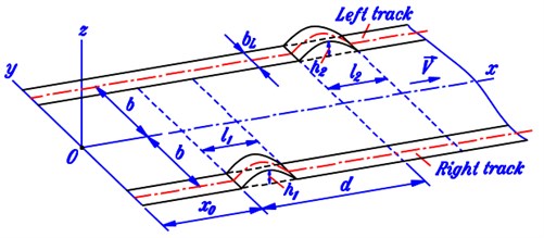
The situation under consideration is that the automobile successively passes a single bump on the right track and another one on the left track after having passed a distance $x_{0}$ measured from the initial time point ( $t =$ 0) as seen in Fig. 5. Profiles of the two bumps are chosen as parabolas whose lengths and heights are ( $l_{1}$ , $h_{1}$ ) and ( $l_{2}$ , $h_{2}$ ), respectively. The distance between the two bumps in the direction of movement is denoted as $d$ .

Fig. 5 is a general description of some cases. If setting $h_{1} =$ 0 or $h_{2} =$ 0, the excitation has the type of a single pulse on the left or the right track only. If taking $d <$ 0, the automobile reaches the bump on the left track before reaching the bump on the right one. If assigning $d =$ 0, $l_{1} = l_{2}$ and $h_{1} = h_{2}$ , we have the situation of a speed bump which crosses over the whole width of road. If choosing $x_{0} =$ 0, the initial point of time ( $t =$ 0) is also the time when the vehicle starts passing the left bump.

Fig. 5Geometrical description of road profile

The input data for numerical computation are taken as:

– Parameters concerned with the automobile [15]: $b =$ 0.90 m, $c =$ 0.60 m, $r_{w} =$ 0.45 m, $b_{L} =$ 0.25 m, $M_{b} =$ 2150 kg, $J_{b} =$ 650 kg.m², $M_{c} =$ 660 kg, $J_{c} =$ 720 kg.m², $k_{T} =$ 250000 N/m, $k_{L} =$ 800000 N/m, $c_{T} =$ 1500 N.s/m, $c_{L} =$ 62000 N.s/m.

– Quantities belonging to the ground and the beam [16]: $k_{S} =$ 48000000 N/m³, $c_{S} =$ 30000 N.s/m³, $E =$ 1.6×10⁹ N/m², $ρ =$ 2500 kg/m³, $L_{B n} =$ 15 m, $b_{B}^{x} =$ 0.45 m, $h_{B} =$ 0.50 m.

– Excitation data (geometries of bumps): $h_{1} =$ 0.10 m, $l_{1} =$ 0.75 m, $h_{2} =$ 0.12 m, $l_{2} =$ 0.80 m, $d =$ 1.0 m.

– Velocity of movement of automobile: $V =$ 10 km/h.

– Parameters involved computation: $t_{m a x} =$ 5 s, $t_{0} =$ 0.5 s, $Δ t =$ 0.0001 s, $N =$ 5 ( $x_{0} = V t$ ).

– Type of pressure distribution in contact areas: cosine.

The obtained results are graphically showed in Fig. 6-9 where the changes in some vibration characteristics with respect to time are plotted. Some comparisons between the two cases of taking and not taking account of wheel separation are given in Figs. 6, 7 and 8.

Fig. 6Linear vibration of automobile body

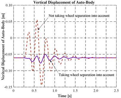
Fig. 7Angular vibration of automobile body

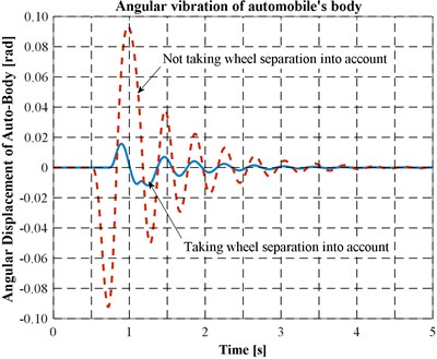
Fig. 8Vertical acceleration of automobile body

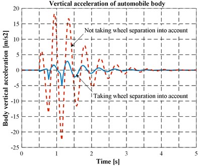
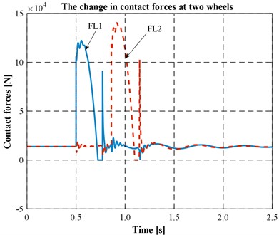
Fig. 9The changes in contact forces at two wheels

It can be seen from the figures that:

a) Differences in behaviour of the mechanical system between the two cases of taking and not taking account of wheel separation are clearly (see Figs. 6, 7 and 8).

b) In the situation of consideration, the amplitude of vibration in the case of not taking wheel separation is greater than the amplitude in the other case. The reason may concern with the ways of transmitting potential energy which has been accumulated by the springs in compressing periods to the body in stretching ones.

c) Wheel separation really occurs in the situation of consideration. This can be identified by flat pieces (on the abscissa) of the curves in Fig. 9. The calculated total times of losing contact are 0.0416 s and 0.0458 s for the right and the left wheels, respectively.

d) After each period of wheel separation, the contact forces rapidly increase (Fig. 9) due to converting kinematic energy of falling into potential energy of the springs.

e) Wheel separation is quite easy to occur. This can be recognized by looking at the values of the parameters which describe the road profile and especially the small value of velocity of movement.

5. Conclusions

The article has created a physical model for considering the quasi-planar lateral vibration of the automobiles with dependent suspensions where all three wheel separation, road deformation and the change in dimension of contact areas have been taken into account. The original differential equations of motion of the vehicle-road coupled system with the presence of a partial differential equation have been transformed into a set of all ordinary differential equations by applying the Bubnov-Galerkin’s method. The authors have also proposed a procedure for numerically solving the transformed differential equations of motion. Vibration of automobile, according to the model introduced above, has been considered in the case in which an automobile moves through two bumps (each bump on one track) of parabolic profiles. The results obtained from numerical computation have proved that the difference between taking and not taking wheel separation into account is significant and the loss of contact is easy to appear while automobiles run on rough roads. Hence, one can affirm the need of taking wheel separation into account in considering vertical vibration of automobiles.

References

Cebon D. Interaction between heavy vehicles and roads. SAE Technical Paper 930001, 1993, https://doi.org/10.4271/930001.

Publisher
Cole D. J. Truck suspension design to minimize road damage. Proceedings of the Institution of Mechanical Engineers, Vol. 210, Issue 22, 1996, p. 95-107.

Publisher
Zhu Q., Ishitobi M. Chaos and bifurcations in a nonlinear vehicle model. Journal of Sound and Vibration, Vol. 275, Issues 3-5, 2004, p. 1136-1146.

Publisher
Yang S., Li S., Lu Y. Investigation on dynamical interaction between a heavy vehicle and road pavement. Vehicle System Dynamics, Vol. 48, Issue 8, 2010, p. 923-944.

Publisher
Li S., Lu Y., Li H. Effects of parameters on dynamics of a nonlinear vehicle-road coupled system. Journal of Computers, Vol. 6, No. 12, 2011, p. 2656-2661.

Publisher
Cheng Y. S., Au E. T. K., Cheung Y. K., Zheng D. Y. On the separation between moving vehicles and bridge. Journal of Sound and Vibration, Vol. 222, Issue 5, 1999, p. 781-801.

Publisher
Baeza L., Ouyang H. Dynamics of a truss structure and its moving-oscillator exciter with separation and impact-reattachment. Proceedings of the Royal Society A: Mathematical, Physical and Engineering Sciences, Vol. 464, Issue 2098, 2008, p. 2517-2533.

Publisher
Stăncioiu D., Ouyang H., Mottershead J. E. Vibration of a continuous beam with multiple elastic supports excited by a moving two-axle system with separation. Meccanica, Vol. 44, Issue 3, 2008, p. 293-303.

Publisher
Zhu D. Y., Zhang Y. H., Ouyang H. A linear complementarity method for dynamic analysis of bridges under moving vehicles considering separation and surface roughness. Computers and Structures, Vol. 154, 2015, p. 135-144.

Publisher
Zhang Y., Zhao H., Lie S. T. A nonlinear multi-spring tire model for dynamic analysis of vehicle-bridge interaction system considering separation and road roughness. Journal of Sound and Vibration, Vol. 436, 2018, p. 112-137.

Publisher
Cuong P. M., Dung T. Q., Nam L. H. Consideration on vibration of automobiles in quarter-car model with the loss of contact taken into account. Journal of Sciences and Technology, Vol. 183, 2017, p. 64-73.

Search CrossRef
Ham V. C., Cuong P. M., Dung T. Q. Consideration of the problem about vibration of automobiles in one-fourth model with taking road deformation and the loss of contact into account. Journal of Vibroengineering, Vol. 22, Issue 4, 2020, p. 945-958.

Publisher
Ham V. C., Cuong P. M., Dung T. Q. Consideration on vibration of automobiles in planar model taking account of the loss of contact. Proceedings of the National Conference on Mechanics and Transportation Engineering, Ho Chi Minh City, Vietnam, Vol. 2, 2017, p. 326-332, (in Vietnamese).

Search CrossRef
Ham V. C., Cuong P. M. Consideration on vibration of automobiles in spatial model with the loss of contact taken into account. International Journal of Applied Engineering Research, Vol. 15, Issue 6, 2020, p. 594-599.

Search CrossRef
Lap V. D. Handbook for looking up technical specifications of automobiles. Le Quy Don Technical University, 2004, (in Vietnamese).

Search CrossRef
Shaopu Y., Liqun C., Shaohua L. Dynamics of Vehicle-Road Coupled Systems. First Edition, Springer-Verlag Berlin Heidelberg, 2015.

Search CrossRef

About this article

Received

20 August 2020

Accepted

29 December 2020

Published

16 January 2021

SUBJECTS

Vibration in transportation engineering

DOI

https://doi.org/10.21595/jve.2020.21670

Keywords

automobile

lateral vibration

loss of contact

wheel separation

quasi-planar model

road deformation

Bubnov-Galerkin’s method

This is an open access article distributed under the Creative Commons Attribution License, which permits unrestricted use, distribution, and reproduction in any medium, provided the original work is properly cited.

Previous article in issue Previous Next article in issue Next

Research article

2021 01 22

Consideration of longitudinal vibration of automobiles in planar model with taking road deformation and loss of contact into account

Ham Vu Cong, Cuong Phung Manh, Dung Tran Quang

Research article

2020 06 30

Consideration of the problem about vibration of automobile in one fourth model with taking road deformation and the loss of contact into account

Ham Vu Cong, Cuong Phung Manh, Dung Tran Quang

Research article

2018 12 31

Simplified theoretical treatment of lateral structural properties under crowd excitation

Yun Dong, Yan An Gao, Ye Zhu, Peng Zhang

Research article

2017 09 26

Laser method of sound emission control from vibrating surfaces of noise road barriers

Zbigniew Motyka

H. Vu Cong, C. Phung Manh, and D. Tran Quang, “Consideration on lateral vibration of automobiles in quasi-planar model with wheel separation and road deformation taken into account,” Journal of Vibroengineering, Vol. 23, No. 1, pp. 256–272, Jan. 2021, https://doi.org/10.21595/jve.2020.21670

Copy Extrica

Copied to clipboard!

TY  - JOUR
DO  - 10.21595/jve.2020.21670
UR  - https://doi.org/10.21595/jve.2020.21670
TI  - Consideration on lateral vibration of automobiles in quasi-planar model with wheel separation and road deformation taken into account
T2  - Journal of Vibroengineering
AU  - Phung Manh, Cuong
AU  - Vu Cong, Ham
AU  - Tran Quang, Dung
PY  - 2021
DA  - 2021/01/16
PB  - JVE International Ltd.
SP  - 256-272
IS  - 1
VL  - 23
SN  - 1392-8716
SN  - 2538-8460
ER  - 

Copy Ris

Copied to clipboard!

@article{Phung_Manh_2021,
	doi = {10.21595/jve.2020.21670},
	url = {https://doi.org/10.21595/jve.2020.21670},
	year = 2021,
	month = {jan},
	publisher = {{JVE} International Ltd.},
	volume = {23},
	number = {1},
	pages = {256--272},
	author = {Cuong Phung Manh and Ham Vu Cong and Dung Tran Quang},
	title = {Consideration on lateral vibration of automobiles in quasi-planar model with wheel separation and road deformation taken into account},
	journal = {Journal of Vibroengineering}
}

Copy Bibtex

Copied to clipboard!

[1]C. Phung Manh, H. Vu Cong, and D. Tran Quang, “Consideration on lateral vibration of automobiles in quasi-planar model with wheel separation and road deformation taken into account,” Journal of Vibroengineering, vol. 23, no. 1, pp. 256–272, Jan. 2021, doi: 10.21595/jve.2020.21670.

Copy IEEE

Copied to clipboard!

Phung Manh, Cuong, Ham Vu Cong, and Dung Tran Quang. “Consideration on Lateral Vibration of Automobiles in Quasi-Planar Model with Wheel Separation and Road Deformation Taken into Account.” Journal of Vibroengineering 23, no. 1 (January 16, 2021): 256–72. https://doi.org/10.21595/jve.2020.21670.

Copy Chicago

Copied to clipboard!

Consideration on lateral vibration of automobiles in quasi-planar model with wheel separation and road deformation taken into account

Abstract

Highlights

1. Introduction

2. Vibration model and differential equations of motion

2.1. Assumptions

2.2. Vibration model of the mechanical system

2.3. Forces acting on the vibration system

2.4. Differential equations of motion of the system

2.4.1. Differential equations of motion of automobile

2.4.2. Differential equation of motion of deformed road

2.5. Simpler cases of differential equations of motion of the system

3. Solving the differential equations of motion

3.1. Transforming the differential equations of motion into ordinary differential equations

3.2. Matrix form of TDEM

3.3. Initial conditions

3.4. Procedure for numerically solving the TDEM

4. Example for illustration

5. Conclusions

References

About this article

Related Articles