Abstract
This paper presents an approach to the problem about vibration of automobiles in one-fourth model where both road deformation and the loss of contact are taken into account. Contact characteristics such as the geometry of the contact area, pressure distribution, the relation between the contact force and the dimensions of the contact area, and therefore the change in dimensions of the contact area with respect to time are mentioned. Deformed road is modeled as an elastic beam which is simply supported at the two ends and lies on Kelvin’s visco-elastic ground. The differential equations of motion for both states of contact and losing contact are unified by introducing a so-called contact state parameter. The partial differential equation among the differential equations of motion of the vehicle-road coupled system is transformed into a system of all ordinary differential equations by applying the Bubnov-Galerkin’s method. A procedure for numerically solving the ordinary differential equations of motion of the vibration system under consideration is proposed and some numerical results for illustration are also presented in the paper.
Highlights
- A new vibration model of vihicle wheel is proposed.
- Both road deformation and wheel separation are taken into account.
- The change in dimension of contact area between wheel with road surface is taken into account.
- Bubnov-Galerkiń s method is applied to get ODEs form original equations of motion where exists a partial differential equation.
1. Introduction
In fact, due to the unevenness of the road surface and the inherent imbalance of parts, a moving automobile is always lying in vibration state and its vertical vibration is a considerable component. Vertical vibration makes the changes in contact pressure and area between the wheels and the road surface. This is the reason of the appearance of dynamic forces acting on the road. When the level of vibration is large enough, the wheels may separate from the road surface and cause the phenomenon of losing contact. This phenomenon is also known as wheel separation, wheel hopping and in this paper, it is called as the loss of contact. The loss of contact results in the loss of control (in terms of speed and direction) and reduces the safety of movement.
Depending on the geometrical and dynamic characteristics of the vehicle itself, the geometry of the road surface and the speed of movement, the loss of contact may occur or not, frequently or infrequently. Conditions for the loss of contact appearing, the limit of speed to avoid losing contact, the rate of time of losing contact over total time of movement, etc. are the factors that deserve to be attended.
Vibration of automobiles in the one-fourth model has been mentioned in [1-7]. In particular, the references [1, 3-5, 7] ignore the deformation of road, and the references [1, 3, 5, 7] do not take into account the phenomenon of losing contact between the wheel and the road surface. The references [2, 6] take account of road deformation but ignore the phenomenon of losing contact. Moreover, these references consider vibration without taking account of the change in dimensions of the contact area or considering different laws of pressure distribution on the contact area. In this paper, the above aspects are mentioned simultaneously.
2. Contact characteristics of the wheel-road couple
Contact characteristics of the wheel-road couple directly involve the formulation of the problem under consideration. The characteristics mentioned here consist of: a) the contact state (in contact or separation state); b) the shape and dimensions of the contact area; c) relations of wheel vertical deformation with the contact area dimensions and the contact force; d) distribution of pressure in the contact area.
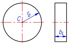
Fig. 1 shows the original dimensions of a wheel with the standard air pressure inside for readiness to be used. The wheel in free state (not subjected to load) is assumed to be exactly rounded. The values of and are called as calculation radius and width, respectively.
Fig. 1The original dimensions of a wheel
2.1. Contact states, geometry of contact area and relations of quantities
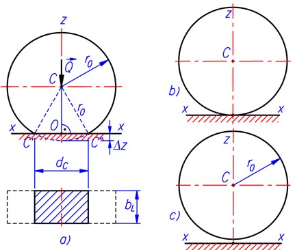
Fig. 2 shows three possible relative positions between a rounded wheel and a road with planar surface. In Fig. 2(a), the wheel lies in contact state with the road surface and it is deformed under the contact force . The shape of the contact area is accepted to be rectangular [6]. For simplicity, we add here two assumptions as follows: a) the off-contact-area part of wheel profile is still exactly rounded with the radius unchanged; b) the width of the wheel is not changed under loading.
With the assumptions mentioned above, the contact area in this relative position has the dimensions as with the length determined as:
where is vertical deformation of the wheel (or tyre).
Once the linearity in behavior of the wheel is accepted, between the contact force and vertical deformation exists the following relation:
where and are stiffness and damping coefficient of the spring-damper couple which represents the elastic and damping properties of the wheel, respectively.
Eqs. (1) and (2) describe the relations of wheel vertical deformation with the contact area length and the contact force.
The second relative position of the wheel-road couple is shown in Fig. 2(b). In this situation, the wheel still lies in the contact state with the road surface but has no deformation. The contact area now reduces to a straight line segment with the length and the contact force is equal to zero.
In Fig. 2(c), the wheel completely loses contact with the road surface and it is not deformed. The contact area is absent and the contact force is also equal to zero.
Because the value of wheel vertical deformation and that of the contact force are simultaneously differ from zero in the first case and simultaneously equal to zero in the two others, so we can unify the equations which express the relation of contact force and wheel vertical deformation for three cases in Fig. 2 as follows:
Parameter in Eq. (3) is taken the value of 0 for cases where 0, 0, and taken the value of 1 in cases 0, 0. Because reflects the state of contact or separation of the wheel-road couple, it is called as the contact state parameter. The introduction of the contact state parameter facilitates making the differential equations of motion of the considered mechanical system as presented in the next section.
In the process of vibration of automobiles, the values of and change with respect to time. They can be determined only by solving the differential equations of motion of the mechanical system under consideration.
Fig. 2Three possible relative positions between a rounded wheel and a planar road surface: a) contact with wheel deformed; b) contact with wheel undeformed; c) no contact
2.2. Distribution of pressure in the contact area
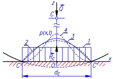
The distribution of pressure in the contact area between the wheel and the road surface depends on many factors such as the geometrical and physical properties of the tire, those of the road and the speed of movement, etc. In fact, the distribution of pressure is very complicated [6]. However, for simplicity in considering vertical vibrations of automobiles, we assume that the distribution of pressure is symmetrical about the coordinate plane , a vertical plane passing through the axle of the wheel as shown in Fig. 3 (where the axis is not described), and moreover, the pressure distribution function does change only in the -direction, not change in the -direction [6, 8].
Fig. 3Pressure distribution laws assumed: 1 – even or rectangle, 2 – parabola, 3 – cosine, 4 –squared cosine)
Accordingly, the pressure distribution function in the contact area can be written in the following form:
where is a time function that reflects the change of pressure with respect to time, is an – variable function which represents the changing of pressure in the direction, is a dimensionless function that depends on the pressure distribution law chosen. The four typical forms of function proposed in the reference [8] are plotted in Fig. 3 and consist of the following laws:
– Even distribution: ;
– Parabola distribution: .
– Cosine distribution: .
– Squared cosine distribution: .
From the force equilibrium in vertical direction, we have:
where is the reaction force from the road upwards to the wheel and:
For rectangle, parabola, cosine and squared cosine distributions, the values of can be obtained from Eq. (6) is , , and , respectively.
The Eqs. (3) and (5) allow to deduce a relation between function and vertical deformation of the wheel:
It is noted that when the wheel is not in contact with the road surface, both and are simultaneously equal to zero. At this time, although the Eq. (7) of has an infinite form 0/0, but the value of contact force is equal to zero.
3. One-fourth vibration model and differential equations of motion
3.1. One-fourth vibration model of automobiles
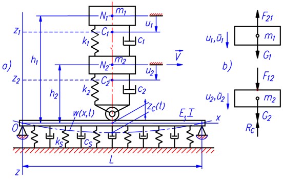
An one-fourth vibration model of automobiles with road deformation taken into account is shown in Fig. 4(a). The automobile is modeled as a vertical vibration system of two masses and the deformable road is model as an elastic beam which is simply supported at the two ends and lies on the Kelvin’s visco-elastic ground.
Vertical vibration of the automobile takes place at the middle of the beam. The effect of automobile movement on vibration is represented by time changing in depth or height of the center point of the contact area due to road roughness. Deformation of the road with respect to time is represented by vibration of the beam.
The beam with the length has uniform rectangular cross-section whose width and height are denoted as and , respectively. Material of the beam is assumed to be homogeneous, isotropic, and has mass density and Young’s modulus .
The position presented in Fig. 4(a) of the vibration system is a so-called natural position where the wheel is in contact with the road surface and all the springs in the model are completely free. In this figure, and are the suspended and unsuspended masses of the vehicle in one-fourth model; is the spring-damper couple which represents the vehicle suspension; is the spring-damper couple representing the elastic and damping properties of the wheel; and are the ground stiffness and damping coefficient per unit area. For simplicity, and are also denoted for the stiffness and damping coefficient of the corresponding spring-damper couples. Vibrations of the two masses and the elastic beam are respectively expressed by the displacement functions , and those are measured from the natural position.
Fig. 4One-fourth vibration model of automobile with road deformation taken into account: a) vibration model and characteristic parameters; b) force diagram of masses
3.2. Differential equations of motion of the vibration system
3.2.1. Differential equations of motion of the automobile
Fig. 4(b) shows the force diagram of the two masses in the mechanical system. On the diagram, are the forces of gravity, and are the resultant force of spring and damping forces in the spring-damper couple . The expressions for and can be written as [4, 6, 8, 9]:
The calculating vertical deformation of the spring representing the tire elasticity (quantity in Eq. (3)) in case the deformation of uneven road is taken into account can be approximately calculated as:
where is the -coordinate of the contact area center (point O in Figs. 2 and 3) measured from the natural position of the nominal road surface, is vertical displacement of the middle cross-section of the beam, and vertical fluctuation (the depth or height of road profile caused by road unevenness) at the contact area center. For simplicity, here we give one more assumption that the effect of road unevenness on vertical deformation of the wheel concerns the center point of the contact area only.
From the vibration model, we can get:
By applying the Newton’s second law to the force diagrams of the two masses in Fig. 4(b), one can obtain:
Using Eqs. (3), (5), (8) and relations , in Eq. (11), we can get the differential equations of motion of the automobile:
In problems about predeterministic vibration of automobiles, the road profile has been predescribed, so that is given as a definite function of time.
3.2.2. Differential equation of motion of the road
The differential equation of motion of the road can be made by considering the equilibrium of a typical beam element which has the length of and locates at the position determined by coordinate as shown in Fig. 5.
Fig. 5Force diagram of a typical beam element in vibration model
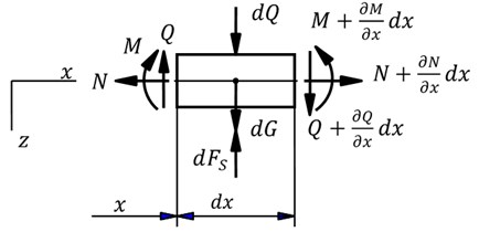
Forces acting on the element include:
– Axial forces , shear forces and bending moments around the y-axis at the left and the right sections.
– The force of gravity , ( – gravitational acceleration).
– Contact force which may exists in the contact area, . If the element is not in contact with the wheel then and are equal to zero.
– Inertial force , .
– Reaction force from the ground , .
The force equilibrium in horizontal and vertical directions, and the moment equilibrium about the center point of the left cross-section of the element combining with neglecting the infinitesimal quantities lead to these equations:
Eq. (14) gives 0 for all , since no external force acts in the -direction.
By substituting Eq. (16) into (15) and noting that [6], one obtains the differential equation of motion of the beam:
where – the Young’s modulus of beam material, – the inertial moment of bending around the -axis of beam cross-section, .
The differential equations of motion of the vehicle-road system are combination of ordinary differential Eqs. (12), (13) and partial differential Eq. (17).
If the loss of contact is not taken into account, the differential equations of motion of the vehicle-road coupled system can be obtained from the equations mentioned above by fixing 1. In case road deformation is neglected, 0 for all and , Eq. (17) is obviously satisfied and the differential equations of motion of the mechanical system reduces to the differential equations of motion Eqs. (12), (13) of the automobile only.
3.3. Transforming the differential equations of motion to a system of all ordinary differential equations (ODE)
In order to obtain the response of the automobile under consideration according to some initial conditions, it is necessary to solve the differential equations of motion mentioned above. Solution given here to reaching that purpose is applying the Bubnov – Galerkin’s method to transform the partial differential Eq. (17) to a system of all ordinary differential equations.
Firstly, the function is approximated by the series of terms as:
where ( 1, 2, ..., ) are time functions to be found, and are functions those satisfy the boundary conditions of the beam, 0, and match the symmetry of about the middle cross-section of the beam.
The functions in Eq. (18) are also linearly independent and have the property of orthogonality as follows:
Substituting the Eq. (18) of and the Eq. (4) of into Eq. (17) leads to the following equation:
In succession, multiplying both two sides of Eq. (20) by the expression: ( 1, 2, ..., ).
Then integrating the two sides of the obtained equation over the entire length of the beam, paying attention to the orthogonality Eq. (19), we obtain a system of ordinary differential equations of the form:
where 1, 2, ..., and:
Because the functions to be determined are , and (1, 2, ..., ), so it is needed to express in Eq. (21) in terms of those unknown functions. The expression of can be obtained by using the Eq. (9) of in Eq. (7):
The expressions of and in Eq. (23) can also be written in terms of the unknown functions by using the Eq. (18) of and Eq. (10):
Substituting Eqs. (24) and (25) into Eq. (23) and putting the result into Eq. (21), then taking some arrangements, we obtain the following equations:
where:
With the Eqs. (24), (25) of and , Eq. (13) is also written in terms of the unknown functions (, and ) as follows:
The original differential Eqs. (12), (13), (17) has now been transformed into a system of all ordinary differential Eq. (12), (28) and (26) those can be called as the transformed differential equations and written in matrix form:
where is the vector of generalized coordinates, is the vector of excitation force and [], [], [] are the mass, damping and stiffness matrices, respectively. The dimension of the two vectors is ()×1 and that of the three matrices is ()×(). Those vectors and matrices can be written in detail as follows:
3.4. Determination of static displacements of the masses and elastic beam
Determination of static displacements of the components is needed in case the vehicle is moving on a completely smooth road when entering a rough road and static displacements are chosen as the corresponding initial conditions to consider vertical vibration of the mechanical system.
Conventionally, the subscript or superscript “0” is used to refer to the values of the corresponding quantities in static state. Because the phenomenon of losing contact and vertical vibrations of the whole system do not occur in static state so 1 and , . At this time, the spring is subjected to the force equal to the total weight of the two masses and , so its static deformation is . As the result, the corresponding length of the contact area can be calculated as:
The values of the quantities in Eq. (22) can be determined according to the pre-chosen law of pressure distribution. Then, we can calculate the value of the matrix [] by using Eqs. (27) and (34), then deduce static displacements based on Eq. (29) as follows:
where is the value of in static state. It is determinned from Eq. (31) by setting = 0.
The displacement expression of the beam is deduced from Eq. (18):
where the values of quantities are last components of vector which has been calculated as in Eq. (36).
3.5. Method for numerically solving the differential equations of motion
Differential Eq. (29) are ODEs with the matrices [] and [] depending on time. Let’s consider the case where the vehicle is moving on a smooth road when entering the rough road and the time point 0 is chosen as the time point of transition between the two road profiles. In this situation, the relevant initial values are taken as those of static state.
The procedure for numerically solving the differential equations of motion Eq. (29) can be described as follows:
1) Assigning values to the quantities , , , , , , , , , , , , , , and the vehicle speed of movement.
2) Describing the profile of road surface as the time functions , .
3) Choosing the pressure distribution function and the value of , the number of terms of the series which is used to approximate function .
4) Selecting the computing time interval [0, ] and the computing time step .
5) Assigning 0, 0, 1, , for starting step of computing.
6) Calculating the values of , I0 and by using Eqs. (35), (6) and (22).
7) Calculating the values of matrices , according to Eqs. (33), (34) and the exciting vector according to Eq. (31).
8) Calculating vectors , and using a known method such as Runge-Kutta’s method.
9) Determining displacement function of the beam according to Eq. (18) and deducing the values of , .
10) Calculating and following one from the two possibilities:
– If 0 then the loss of contact does not occur, so 1. At this point of time, it is needed to calculate the values of , , .
– If 0 then the loss of contact occurs or starts to occur and 0. Now 0 and the terms concerning in Eq. (26) are absent and 0.
11) Assigning , and repeating the process of calculation from step 7. The process of calculation ends when reaching the condition .
At the end of the process of calculation, we obtain the following functions , , , , …, together with their first and second derivatives. The displacement function which describes the road deformation at each time point is determined by applying Eq. (16).
4. Some results from numerical computation
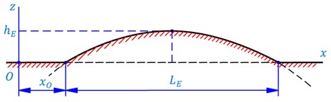
This section presents some typical results obtained from numerical computation. The situation under consideration is that the automobile is moving on a completely smooth road surface with a constant velocity when passing a bump that has the profile of parabolic type as shown in Fig. 6. In the figure, the origin corresponds to the initial time (0) of the process of computation, – the distance of moving before the vehicle enters the bump ( the corresponding time), and – the height and the length (in direction of movement) of the bump, respectively.
Fig. 6Road profile of parabolic type and geometrical characteristics
The input data of consideration are taken as follows:
– The values of parameters concerned with the vehicle (automobile): 1500 kg, 246000 N/m, 1500 N.s/m, 500 kg, 800000 N/m, 62000 N.s/m, 0.25 m, 0.45 m.
– The data belonging to Kelvin’s visco-elastic ground and the elastic beam: 48×106 N/m2, 30000 N.s/m, 1.6×10⁹ Pa, 20 m, 0.45 m, 0.50 m.
– The values of parameters concerned with the bump the time interval of consideration () and the number of terms of the series used to approximate : 0.80 m, 0.15 m, 0.5 s, 5 s, 5.
The above value of is taken after a process of considering on convergence of results has been carried out.
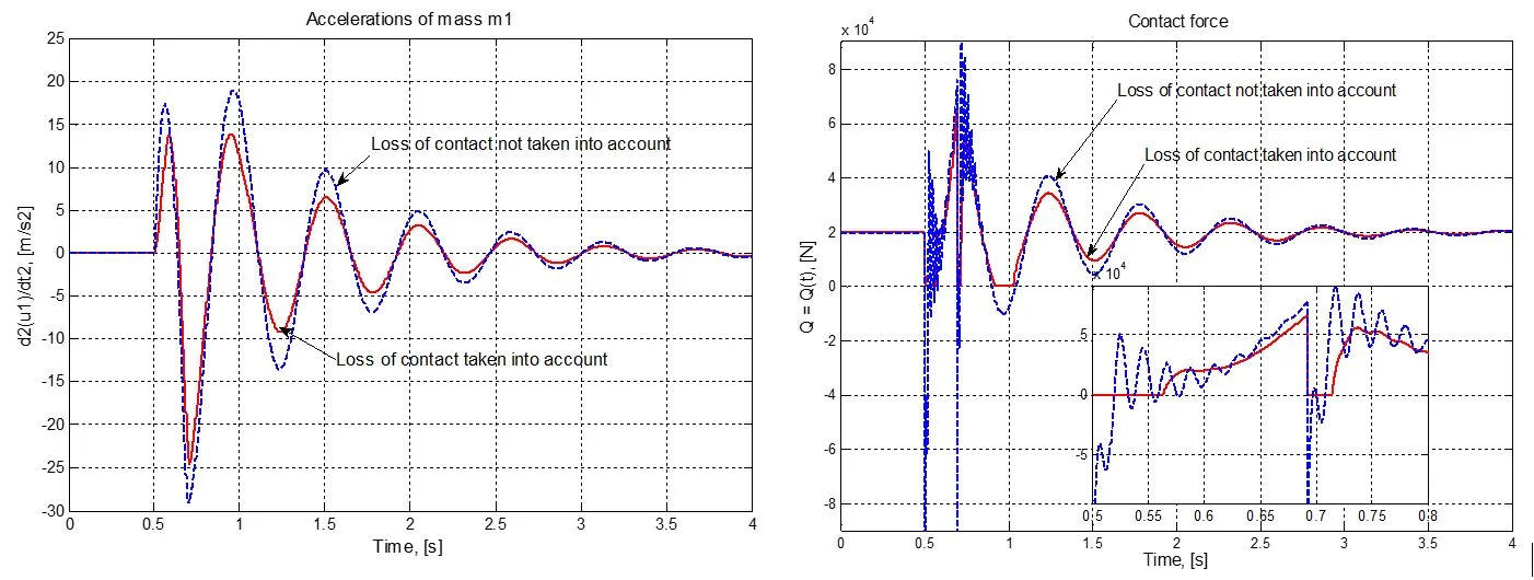
The results will be given in both graphical and table forms. Two considerable quantities are the acceleration of the vehicle body (which is represented by mass ) and the contact force (ie. and ). The results in case of taking the loss of contact into account are compared to the corresponding results in case of not taking the loss of contact into account.
The plots in Fig. 7 and Fig. 8 present the change in acceleration of the vehicle body and the change in contact force with respect to time in case the automobile moves with constant velocity 15 km/h. The plot with some flat pieces lying on the abscissa in Fig. 7 shows that the loss of contact really appears in the conditions of consideration. The clear differences of the two curves in both plots prove the need of taking the loss of contact into account.
Fig. 7The change in acceleration of the vehicle body, u¨1=u¨1(t)
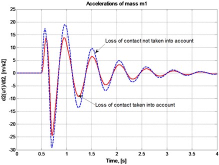
Fig. 8The change in contact force, Q=Qt
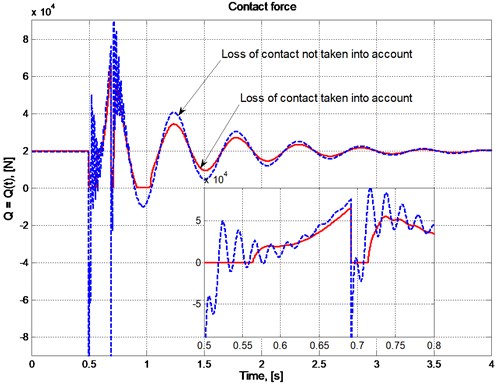
Table 1 shows the root-mean-squared values of the vehicle acceleration and the contact force () versus the velocity of movement () in both cases of taking (, ) and not taking (, ) the loss of contact into account. The total time () of losing contact in each considered case is also given in the Table 1.
The data in the above table also show the significant differences between the two cases of taking and not taking the loss of contact into account. However, the law of changing in values of the five quantities considered above is not clear. It may be concerned with the excitation – response relation and needs some consideration in more detail.
Table 1Analysis results
[km/h] | 5 | 10 | 15 | 20 | 25 | 30 |
, [m/s2] | 4.1897 | 5.9293 | 4.5593 | 3.7019 | 3.9686 | 4.2066 |
, [m/s2] | 4.6052 | 7.2719 | 6.2176 | 5.2483 | 4.5286 | 3.9934 |
, [N] | 20860 | 21677 | 20904 | 20657 | 21025 | 21441 |
, [N] | 21052 | 22877 | 22605 | 22948 | 23841 | 25135 |
, [s] | 0.2111 | 0.2736 | 0.1955 | 0.0976 | 0.1422 | 0.2370 |
5. Conclusions
The article has modeled and expressed the relations of parameters which characterize the contact between the wheel of an automobile and the road surface. A description of the change in dimensions of the contact area is mentioned and some typical laws of pressure distribution are given. A physical model of the vehicle-road coupled system is introduced where the one-fourth model of the vehicle is applied, the road deformation and the phenomenon of losing contact are taken into account. The use of contact state parameter allows to unify the differential equations of motion in both states of contact and losing contact. The differential equations of motion which include a partial differential equation are transformed into a system of all ordinary differential equations by applying the Bubnov-Galerkin’s method. A procedure for numerically solving the transformed differential equations is given and some typical numerical results are also presented. The results have showed significant differences in behaviour of the mechanical system between the two cases taking and not taking the loss of contact into account. Hence, taking the loss of contact into account in consideration of problems on vibration of automobiles is needed.
References
-
Agostinacchio M., Ciampa D., Olita S. The vibration induced by surface irregularities in road pavement – a Matlab approach. Journal European Transport Research Review, Vol. 6, Issue 3, 2014, p. 276-275.
-
Hu D., Yan Y., Li Qun C., Shao Pu Y. Vibration of vehicle – pavement coupled system based on a nonlinear foundation. Journal of Sound and Vibration, Vol. 333, Issue 24, 2014, p. 6623-6636.
-
Mahmoud R., Atanu B. Passive suspension modelling and analysis of a full – car model. International Journal of Advanced Science Engineering Technology, Vol. 3, Issue 2, 2013, p. 250-261.
-
Cuong P. M., Dung T. Q. Consideration of vibration of automobile in quarter model with the loss of contact taken into account. Journal of Sciences and Engineering, 2017, p. 39-48.
-
Jazar Reza N. Vehicle Roll Dynamics. Vehicle Dynamics: Theory and Application. Springer, Boston, 2008, p. 665-725.
-
Yang Shaopu, Chen Liqun, Li Shaohua Dynamics of Vehicle-Road Coupled System. Springer, 2015.
-
Waters T. P., Hyn Y., Brennan M. J. The effect of dual – rate suspension damping on vehicle response to transient road inputs. Journal of Vibration and Acoustic, February, Vol. 31, Issue 1, 2009, p. 011004.
-
Ham C. V., Dung D. N. Identification of contact characteristics in the problem on dynamic interaction between vehicles and roads. Vietnam Journal of Transportation, 2016, p. 108-110.
-
Ham C. V., Dung D. N. Consideration of the phenomenon losing contact between vehicle’s wheels and road surfaces caused by vertical vibrations. Proceedings of the National Conference on Engineering Mechanics, Da Nang, Vietnam, August, Vol. 2, 2015, p. 108-115.
-
Dieter S., Hiller M., Baradini R. Vehicle Dynamics, Modeling and Simulation. Springer, Berlin, 2018.
-
Singiresu S. R. Mechanical Vibrations. 5th Edition, Prentice Hall, 2011.
Cited by
About this article

