Consideration of longitudinal vibration of automobiles in planar model with taking road deformation and loss of contact into account

Vu Cong, Ham; Phung Manh, Cuong; Tran Quang, Dung

doi:10.21595/jve.2021.21575

Journal of Vibroengineering

Browse Journal

Submit article

Published: 22 January 2021

Check for updates

Consideration of longitudinal vibration of automobiles in planar model with taking road deformation and loss of contact into account

Ham Vu Cong¹

Cuong Phung Manh²

Dung Tran Quang³

^{1, 2, 3}Faculty of Mechanics, Le Quy Don Technical University, Ha Noi, Vietnam

Corresponding Author:

Cuong Phung Manh

Cite the article Download PDF

Downloads 854

Abstract

This article considers longitudinal planar vibration of a two-axle automobile moving linearly with a constant velocity and subjected to pre-deterministic kinematic excitation caused by the rough road surface. The automobile is modeled as a vibration system which has three masses and four degrees of freedom. The deformed road is modeled as an elastic beam which is simply supported at the two ends and lying on Kelvin’s visco-elastic ground. The change in dimensions of the contact areas is considered. The loss of contact between the wheels and the road surface is taken into account by producing the contact state parameters in the differential equations of motion of the vibration system. The partial differential equation which describes the motion of deformed road is then transformed into a set of all ordinary differential equations by applying the Bubnov-Galerkin’s method. Some typical results coming from numerical consideration are also presented in the article.

Consideration of longitudinal vibration of automobiles in planar model with taking road deformation and loss of contact into account

Highlights

A longitudinal vibration planar model of the vehicle-road coupled system is proposed.
Both road deformation and wheel separation are considered.
The change in dimension of contact area between wheel with road surface is taken into account.
The different equations of motion are transformed into the system of all ODEs by applying the Bubnov-Galerkin's method.
Vibration of the vehicle is considered in four different cases which is taking road deformation and wheel separation into account or not.

1. Introduction

When an automobile moves on rough roads, vertical vibrations appear as an inherent property. If the level of vibration exceeds a definite threshold, the wheels of the automobile may separate from the road and this phenomenon is called as the loss of contact, or the wheel separation in some documents. The loss of contact reduces controllability of the automobile both in velocity and direction, and therefore, the safety of movement.

In many books and papers concerned with the vibration of automobiles, the loss of contact is either disregarded such as in the references from [1-13] or although regarded but all spring-damper couples which represent the wheels has the lower end consistently clamped to the road surface as in [14]. These physical models are widely applied and help scientists to gain a lot of significant results, but obviously not authentic. It is needed to propose other models which have the authenticity higher.

Recently, the authors of this own article have started investigating into vertical vibration of automobiles with taking account of wheel separation or/and road deformation. The loss of contact is taken into account by introducing the so-called contact state parameters while the road deformation is taken into account by applying the models of elastic beam or rectangular plate on Kelvin's visco-elastic ground. In papers [15, 16], the one-fourth model is applied and the loss of contact is taken into account, but only the article [16] takes account of the road deformation. In the article [17], longitudinal vibration of automobiles is considered in the planar model (a half-car or one-second model), the loss of contact is also taken into account, but the road deformation is not regarded. This paper continues to consider longitudinal vibration of automobiles in the planar model where the loss of contact is taken into account by using two contact state parameters and the road deformation is taken into account by applying the models of the elastic beam on Kelvin's visco-elastic ground.

2. Formulation of the problem

2.1. Assumptions

Vibration model of the vehicle-road coupled system is made with these assumptions:

– Automobile under consideration has the body and two axles absolutely rigid and move linearly with a constant velocity.

– Dynamic behavior of all spring-damper couples in the systems is linear.

– Contact area (if exists) between each wheel and the road surface is a rectangle whose dimension in the direction of vehicle axle is unchanged while loaded.

– The road profile is assumed to be predeterministic.

2.2. Contact characteristics between the wheel and the road

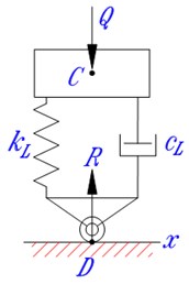
Fig. 1 shows a round wheel that is lying in contact state with the road surface and its vibration model. In the figure, $r_{w}$ is the radius of the wheel; $b_{L}$ – the width of the tyre, also the width of the contact area if exists; $k_{L}$ , $c_{L}$ – the wheel string-damper couple which represents the dynamic behavior of the wheel in vertical direction; $C$ - center of the wheel; $Q$ – vertical load applied on the wheel axle; $R$ – reaction force from the road; $∆ z_{L}$ – vertical compress deformation of the wheel or the spring representing its elasticity; $d_{c}$ – the length of the contact area; $D$ – the expected contact point between the road surface and the wheel. In general, $D$ is the shadow (in vertical direction) of the wheel center onto the road surface; if the contact state between the wheel and the road surface exists, $D$ is also the center of the contact area.

Fig. 1a) Contact characteristics and b) vibration model of a deformed wheel

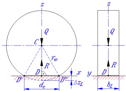
a)

b)

Assuming that the off-contact-area part of the wheel profile is still exactly rounded with the radius unchanged, we can get the relation between the length of contact area and vertical deformation of the wheel:

1

d_{c} = 2 \sqrt{r_{w}^{2} - (r_{w} - Δ z_{L})^{2}} .

Let $F_{L}$ be the resultant of spring and damping forces in the wheel spring-damper couple. From the equilibrium condition of forces acting in the wheel model one can get $Q = R = F_{L}$ . The value of $F_{L}$ can be expressed in term of vertical compress deformation of the wheel $∆ z_{L}$ ( $∆ z_{L}$ is also the spring which represents the wheel) as:

2

F_{L} = k_{L} (Δ z_{L}) + c_{L} \frac{d (Δ z_{L})}{d t} .

If the loss of contact really appears or starts to appear, the wheel is not deformed and the values of $Δ z_{L}$ , $d_{c}$ and $F_{L}$ are all equal to zero.

Now if we redefine $Δ z_{L}$ as the difference in vertical displacements of points $D$ and $C$ , i.e. $Δ z_{L} = u_{D} - u_{C}$ , noting that both road deformation and wheel separation are taken into account, then the expression in the right side of Eq. (2) can be used to verify if the loss of contact occurs or not. This expression can be called as the verifying value of contact force and denoted as ${\bar{F}}_{L}$ , so that:

3

{\bar{F}}_{L} = k_{L} (u_{D} - u_{C}) + c_{L} ({\dot{u}}_{D} - {\dot{u}}_{C}) .

It is obvious that if ${\bar{F}}_{L} \geq 0$ , the wheel still lies in the contact state with the road and ${\bar{F}}_{L}$ is also the resultant force of the wheel spring-damper couple. If ${\bar{F}}_{L} < 0$ , the wheel separates from the road and the resultant force of the wheel spring-damper couple is equal to zero. According to this reasoning, we introduce the so-called contact state parameter which is denoted as s and taken value as $s =$ 1 if ${\bar{F}}_{L} \geq 0$ and $s =$ 0 if ${\bar{F}}_{L} < 0$ . The formula for the resultant force of the wheel spring-damper couple in all three different states of relative position of the wheel-road couple (really contacting, starting to separate or contact, and really losing contact) now can be uniquely written as follows:

4

F_{L} = s {\bar{F}}_{L} = s [k_{L} (u_{D} - u_{C}) + c_{L} ({\dot{u}}_{D} - {\dot{u}}_{C})] .

In order to distinguish the front and the rear wheels later, we will use subscripts or superscripts “1” and “2” respectively, such as $k_{L j}$ , $c_{L j}$ , $F_{L j}$ , $s_{j}$ , $d_{c j}$ , $∆ z_{L j}$ , etc. ( $j =$ 1, 2).

2.3. Vibration model of the vehicle-road coupled system

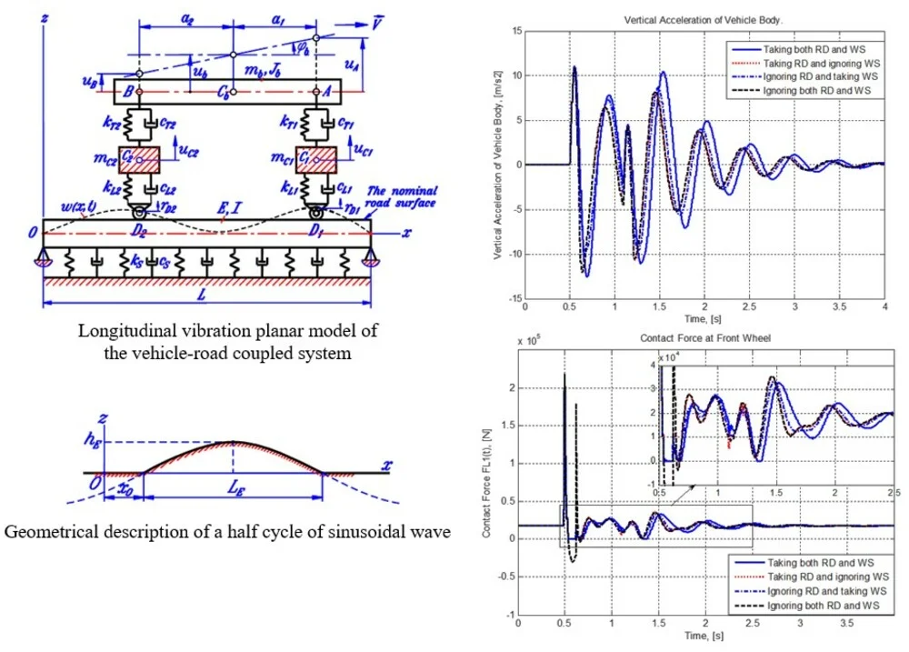
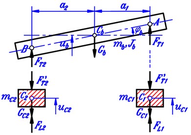
Basing on the construction of two-axle automobiles and the assumptions mentioned above, we can make the longitudinal planar vibration model of an automobile taking road deformation into account as shown in Fig. 2. The vehicle is modeled as a vibration system of three masses corresponding to the body and the two axles while the deformable road is modeled as an homo-geneous elastic beam lying on the Kelvin’s visco-elastic ground. Fig. 2 describes the mechanical system under consideration in the so-called natural position in which all the springs are completely free and the road lies in the contact state with the two wheels.

Fig. 2Longitudinal vibration planar model of the vehicle-road coupled system

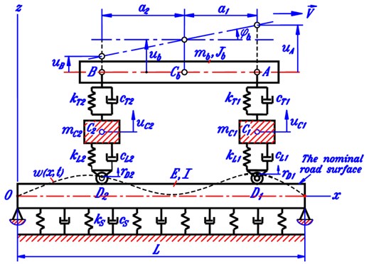
Here are some explanations for Fig. 2:

$C_{b}$ , $C_{1}$ , $C_{2}$ – centers of gravity of the body, the front and the rear axles, respectively;

$A$ , $B$ – connection points of suspension spring-damper couples to the vehicle body;

$m_{b}$ , $J_{b}$ , $m_{C 1}$ , $m_{C 2}$ – inertial characteristics of the vehicle body and the two axles;

$\{k_{T 1}, c_{T 1}\}$ , $\{k_{T 2}, c_{T 2}\}$ – suspension spring-damper couples at the front and the rear axles;

$\{k_{L 1}, c_{L 1}\}$ , $\{k_{L 2}, c_{L 2}\}$ – wheel spring-damper couples at the front and the rear axles;

$\{k_{S}, c_{S}\}$ – stiffness and damping coefficient of Kelvin’s visco-elastic ground;

$a_{1}$ , $a_{2}$ – distances in horizontal direction from the center of gravity of the vehicle body to the front and the rear axles;

$w = w (x, t)$ – displacement function of the beam representing the deformed road;

$u_{b}$ , $φ_{b}$ – vertical and angular displacements of the vehicle body;

$u_{C 1}$ , $u_{C 2}$ – vertical displacements of the front and the rear axles;

$u_{A}$ , $u_{B}$ – vertical displacements of points $A$ and $B$ ;

$r_{D 1}$ , $r_{D 2}$ – representatives of the heights (or depths) at the expected contact points $D_{1}$ , $D_{2}$ from the nominal road surface due to the road roughness.

It is noted that the displacements $u_{b}$ , $φ_{b}$ , $u_{C 1}$ , $u_{C 2}$ are measured from the natural position of three masses (vehicle body and two axles).

2.4. Determination of forces acting on the automobile

Fig. 3 shows the force diagrams of three masses in vibration model after freeing them. In the figure, $G_{b}$ , $G_{C 1}$ , $G_{C 2}$ are the gravitational forces of three masses; $F_{T 1}$ , $F_{T 2}$ , $F_{T 1}^{'}$ , $F_{T 2}^{'}$ – the resultant forces of the suspension spring-damper couples; $F_{L 1}$ , $F_{L 2}$ - the resultant forces of the wheel spring-damper couples, or the contact forces for simpliciy. Subscripts $b$ , 1 and 2 used here imply that the concerned quantity belongs to or concerns with the vehicle body, the front and the rear axles, respectively.

Fig. 3Force diagrams of vehicle body and two axles

The forces in Fig. 3 can be expressed as:

5

G_{b} = m_{b} g, G_{C 1} = m_{C 1} g, G_{C 2} = m_{C 2} g,

F_{T 1} = F'_{T 1} = k_{T 1} (u_{C 1} - u_{A}) + c_{T 1} ({\dot{u}}_{C 1} - {\dot{u}}_{A}),

F_{T 2} = F'_{T 2} = k_{T 2} (u_{C 2} - u_{B}) + c_{T 2} ({\dot{u}}_{C 2} - {\dot{u}}_{B}),

F_{L 1} = s_{1} {\bar{F}}_{L 1} = s_{1} [k_{L 1} (u_{D 1} - u_{C 1}) + c_{L 1} ({\dot{u}}_{D 1} - {\dot{u}}_{C 1})],

F_{L 2} = s_{2} {\bar{F}}_{L 2} = s_{2} [k_{L 2} (u_{D 2} - u_{C 2}) + c_{L 2} ({\dot{u}}_{D 2} - {\dot{u}}_{C 2})] .

Vertical displacements $u_{A}$ , $u_{B}$ , $u_{D 1}$ , $u_{D 2}$ in Eq. (5) can be calculated as:

6

u_{A} = u_{b} + a_{1} φ, u_{B} = u_{b} - a_{2} φ, u_{D 1} = w_{D 1} + r_{D 1}, u_{D 2} = w_{D 2} + r_{D 2},

where $w_{D 1} = w (x, t) | |_{x = x_{D 1}}$ , $w_{D 2} = w (x, t) | |_{x = x_{D 2}}$ are vertical displacements at points $D_{1}$ and $D_{2}$ of the beam which represents the deformed road.

Substituting Eq. (6) into Eq. (5) one can get the expressions of resultant forces in suspension and wheel spring-damper couples:

7

F_{T 1} = F'_{T 1} = k_{T 1} [u_{C 1} - (u_{b} + a_{1} φ_{b})] + c_{T 1} [{\dot{u}}_{C 1} - ({\dot{u}}_{b} + a_{1} {\dot{φ}}_{b})],

F_{T 2} = F'_{T 2} = k_{T 2} [u_{C 2} - (u_{b} - a_{2} φ_{b})] + c_{T 2} [{\dot{u}}_{C 2} - ({\dot{u}}_{b} - a_{2} {\dot{φ}}_{b})],

F_{L 1} = s_{1} [k_{L 1} (w_{D 1} + r_{D 1} - u_{C 1}) + c_{L 1} ({\dot{w}}_{D 1} + {\dot{r}}_{D 1} - {\dot{u}}_{C 1})],

F_{L 2} = s_{2} [k_{L 2} (w_{D 2} + r_{D 2} - u_{C 2}) + c_{L 2} ({\dot{w}}_{D 2} + {\dot{r}}_{D 2} - {\dot{u}}_{C 2})] .

2.5. Differential equations of motion of the mechanical system

2.5.1. Differential equations of motion of the vehicle

By writing the dynamic equations of three masses in Fig. 3 then using the Eq. (7) of forces and taking some needed arrangements, we can get the differential equations of motion of the vehicle as follows:

8

\{\begin{array}{l} m_{b} {\ddot{u}}_{b} + (c_{T 1} + c_{T 2}) {\dot{u}}_{b} + (c_{T 1} a_{1} - c_{T 2} a_{2}) {\dot{φ}}_{b} - c_{T 1} {\dot{u}}_{C 1} - c_{T 2} {\dot{u}}_{C 2} \\ + (k_{T 1} + k_{T 2}) u_{b} + (k_{T 1} a_{1} - k_{T 2} a_{2}) φ_{b} - k_{T 1} u_{C 1} - k_{T 2} u_{C 2} = - m_{b} g, \\ J_{b} {\ddot{φ}}_{b} + (c_{T 1} a_{1} - c_{T 2} a_{2}) {\dot{u}}_{b} + (c_{T 1} a_{1}^{2} + c_{T 2} a_{2}^{2}) {\dot{φ}}_{b} - c_{T 1} a_{1} {\dot{u}}_{C 1} + c_{T 2} a_{2} {\dot{u}}_{C 2} \\ + (k_{T 1} a_{1} - k_{T 2} a_{2}) u_{b} + (k_{T 1} a_{1}^{2} + k_{T 2} a_{2}^{2}) φ_{b} - k_{T 1} a_{1} u_{C 1} + k_{T 2} a_{2} u_{C 2} = 0, \\ m_{C 1} {\ddot{u}}_{C 1} - c_{T 1} {\dot{u}}_{b} - c_{T 1} a_{1} {\dot{φ}}_{b} + (c_{T 1} + s_{1} c_{L 1}) {\dot{u}}_{C 1} - k_{T 1} u_{b} - k_{T 1} a_{1} φ_{b} \\ + (k_{T 1} + s_{1} k_{L 1}) u_{C 1} = - m_{C 1} g + s_{1} [k_{L 1} (w_{D 1} + r_{D 1}) + c_{L 1} ({\dot{w}}_{D 1} + {\dot{r}}_{D 1})], \\ m_{C 2} {\ddot{u}}_{C 2} - c_{T 2} {\dot{u}}_{b} + c_{T 2} a_{2} {\dot{φ}}_{b} + (c_{T 2} + s_{2} c_{L 2}) {\dot{u}}_{C 2} - k_{T 2} u_{b} + k_{T 2} a_{2} φ_{b} \\ + (k_{T 2} + s_{2} k_{L 2}) u_{C 2} = - m_{C 2} g + s_{2} [k_{L 2} (w_{D 2} + r_{D 2}) + c_{L 2} ({\dot{w}}_{D 2} + {\dot{r}}_{D 2})] . \end{array}

2.5.2. Differential equation of motion of the deformed road

As presented above, the deformed road is modeled as homogeneous elastic beam that lies on Kelvin’s visco-elastic ground. Additionally, the beam is simply supported at the two ends has the length of $L$ , the rectangular cross-section with the width $b_{B}$ and the height $h_{B}$ . Vertical displacement of the beam is a function of the $x$ -coordinate and time $t$ , ie. $w = w (x, t)$ .

By considering the equilibrium of a typical beam element, we can obtain the differential equation of motion of the beam which represents the deformed road as follows [16]:

9

ρ h_{B} \frac{\partial^{2} w (x, t)}{\partial t^{2}} + c_{S} \frac{\partial w (x, t)}{\partial t} + k_{S} w (x, t) + \frac{E I}{b_{B}} \frac{\partial^{4} w (x, t)}{\partial x^{4}} + p (x, t) = - ρ h_{B} g .

In Eq. (9), $ρ$ and $E$ – mass density and Young’s module of beam material; $I$ – bending inertial moment of beam cross-section ( $I = b_{B} h_{B}^{3} / 12$ ); $g$ – gravitational acceleration and $p (x, t)$ – function of pressure distribution in the contact areas. Function $p (x, t)$ is assumed unchanged in $y$ -direction and exists in wheel-beam contact areas only.

Solution $w = w (x, t)$ of Eq. (9) should be satisfied the boundary conditions:

10

w (x, t) | |_{x = 0} = w (x, t) | |_{x = L} = 0 .

The differential equations of motion of the vehicle-road coupled system are the combination of four ordinary differential Eq. (8) and partial differential Eq. (9).

2.6. Simpler particular cases of the differential equations of motion

2.6.1. The case of ignoring road deformation

In case the road deformation is ignored, we have $w (x, t) =$ 0 for all $x$ and $t$ . Moreover, it can be assumed that $k_{S} = c_{S} = \infty$ and Eq. (9) becomes an identity. The differential equations of motion of the vehicle-road coupled system reduce to those of the vehicle only and have the form as follows:

11

\{\begin{array}{l} m_{b} {\ddot{u}}_{b} + (c_{T 1} + c_{T 2}) {\dot{u}}_{b} + (c_{T 1} a_{1} - c_{T 2} a_{2}) {\dot{φ}}_{b} - c_{T 1} {\dot{u}}_{C 1} - c_{T 2} {\dot{u}}_{C 2} \\ + (k_{T 1} + k_{T 2}) u_{b} + (k_{T 1} a_{1} - k_{T 2} a_{2}) φ_{b} - k_{T 1} u_{C 1} - k_{T 2} u_{C 2} = - m_{b} g, \\ J_{b} {\ddot{φ}}_{b} + (c_{T 1} a_{1} - c_{T 2} a_{2}) {\dot{u}}_{b} + (c_{T 1} a_{1}^{2} + c_{T 2} a_{2}^{2}) {\dot{φ}}_{b} - c_{T 1} a_{1} {\dot{u}}_{C 1} + c_{T 2} a_{2} {\dot{u}}_{C 2} \\ + (k_{T 1} a_{1} - k_{T 2} a_{2}) u_{b} + (k_{T 1} a_{1}^{2} + k_{T 2} a_{2}^{2}) φ_{b} - k_{T 1} a_{1} u_{C 1} + k_{T 2} a_{2} u_{C 2} = 0, \\ m_{C 1} {\ddot{u}}_{C 1} - c_{T 1} {\dot{u}}_{b} - c_{T 1} a_{1} {\dot{φ}}_{b} + (c_{T 1} + s_{1} c_{L 1}) {\dot{u}}_{C 1} - k_{T 1} u_{b} - k_{T 1} a_{1} φ_{b} \\ + (k_{T 1} + s_{1} k_{L 1}) u_{C 1} = - m_{C 1} g + s_{1} (k_{L 1} r_{D 1} + c_{L 1} {\dot{r}}_{D 1}), \\ m_{C 2} {\ddot{u}}_{C 2} - c_{T 2} {\dot{u}}_{b} + c_{T 2} a_{2} {\dot{φ}}_{b} + (c_{T 2} + s_{2} c_{L 2}) {\dot{u}}_{C 2} - k_{T 2} u_{b} + k_{T 2} a_{2} φ_{b} \\ + (k_{T 2} + s_{2} k_{L 2}) u_{C 2} = - m_{C 2} g + s_{2} (k_{L 2} r_{D 2} + c_{L 2} {\dot{r}}_{D 2}) . \end{array}

2.6.2. The case of disregarding the loss of contact

If the wheels are assumed to lie in the consistent contact state with the road surface, we have $s_{1} = s_{2} =$ 1 at every point of time. In this case, Eq. (9) is still used with no change and the differential equations of motion of the vehicle can be deduced from Eq. (8) by setting $s_{1} = s_{2} =$ 1:

12

\{\begin{array}{l} m_{b} {\ddot{u}}_{b} + (c_{T 1} + c_{T 2}) {\dot{u}}_{b} + (c_{T 1} a_{1} - c_{T 2} a_{2}) {\dot{φ}}_{b} - c_{T 1} {\dot{u}}_{C 1} - c_{T 2} {\dot{u}}_{C 2} \\ + (k_{T 1} + k_{T 2}) u_{b} + (k_{T 1} a_{1} - k_{T 2} a_{2}) φ_{b} - k_{T 1} u_{C 1} - k_{T 2} u_{C 2} = - m_{b} g, \\ J_{b} {\ddot{φ}}_{b} + (c_{T 1} a_{1} - c_{T 2} a_{2}) {\dot{u}}_{b} + (c_{T 1} a_{1}^{2} + c_{T 2} a_{2}^{2}) {\dot{φ}}_{b} - c_{T 1} a_{1} {\dot{u}}_{C 1} + c_{T 2} a_{2} {\dot{u}}_{C 2} \\ + (k_{T 1} a_{1} - k_{T 2} a_{2}) u_{b} + (k_{T 1} a_{1}^{2} + k_{T 2} a_{2}^{2}) φ_{b} - k_{T 1} a_{1} u_{C 1} + k_{T 2} a_{2} u_{C 2} = 0, \\ m_{C 1} {\ddot{u}}_{C 1} - c_{T 1} {\dot{u}}_{b} - c_{T 1} a_{1} {\dot{φ}}_{b} + (c_{T 1} + c_{L 1}) {\dot{u}}_{C 1} - k_{T 1} u_{b} - k_{T 1} a_{1} φ_{b} + (k_{T 1} + k_{L 1}) u_{C 1} \\ = - m_{C 1} g + [k_{L 1} (w_{D 1} + r_{D 1}) + c_{L 1} ({\dot{w}}_{D 1} + {\dot{r}}_{D 1})], \\ m_{C 2} {\ddot{u}}_{C 2} - c_{T 2} {\dot{u}}_{b} + c_{T 2} a_{2} {\dot{φ}}_{b} + (c_{T 2} + c_{L 2}) {\dot{u}}_{C 2} - k_{T 2} u_{b} + k_{T 2} a_{2} φ_{b} + (k_{T 2} + k_{L 2}) u_{C 2} \\ = - m_{C 2} g + [k_{L 2} (w_{D 2} + r_{D 2}) + c_{L 2} ({\dot{w}}_{D 2} + {\dot{r}}_{D 2})] . \end{array}

2.6.3. The case of ignoring both the road deformation and the loss of contact

If both the road deformation and the loss of contact are ignored, the differential equations of motion of the vehicle-road coupled system reduce to those of the vehicle in which $s_{1} = s_{2} =$ 1 and $w_{D 1} = w_{D 2} = {\dot{w}}_{D 1} = {\dot{w}}_{D 2} =$ 0:

13

\{\begin{array}{l} m_{b} {\ddot{u}}_{b} + (c_{T 1} + c_{T 2}) {\dot{u}}_{b} + (c_{T 1} a_{1} - c_{T 2} a_{2}) {\dot{φ}}_{b} - c_{T 1} {\dot{u}}_{C 1} - c_{T 2} {\dot{u}}_{C 2} \\ + (k_{T 1} + k_{T 2}) u_{b} + (k_{T 1} a_{1} - k_{T 2} a_{2}) φ_{b} - k_{T 1} u_{C 1} - k_{T 2} u_{C 2} = - m_{b} g, \\ J_{b} {\ddot{φ}}_{b} + (c_{T 1} a_{1} - c_{T 2} a_{2}) {\dot{u}}_{b} + (c_{T 1} a_{1}^{2} + c_{T 2} a_{2}^{2}) {\dot{φ}}_{b} - c_{T 1} a_{1} {\dot{u}}_{C 1} + c_{T 2} a_{2} {\dot{u}}_{C 2} \\ + (k_{T 1} a_{1} - k_{T 2} a_{2}) u_{b} + (k_{T 1} a_{1}^{2} + k_{T 2} a_{2}^{2}) φ_{b} - k_{T 1} a_{1} u_{C 1} + k_{T 2} a_{2} u_{C 2} = 0, \\ m_{C 1} {\ddot{u}}_{C 1} - c_{T 1} {\dot{u}}_{b} - c_{T 1} a_{1} {\dot{φ}}_{b} + (c_{T 1} + c_{L 1}) {\dot{u}}_{C 1} - k_{T 1} u_{b} - k_{T 1} a_{1} φ_{b} + (k_{T 1} + k_{L 1}) u_{C 1} \\ = - m_{C 1} g + (k_{L 1} r_{D 1} + c_{L 1} {\dot{r}}_{D 1}), \\ m_{C 2} {\ddot{u}}_{C 2} - c_{T 2} {\dot{u}}_{b} + c_{T 2} a_{2} {\dot{φ}}_{b} + (c_{T 2} + c_{L 2}) {\dot{u}}_{C 2} - k_{T 2} u_{b} + k_{T 2} a_{2} φ_{b} + (k_{T 2} + k_{L 2}) u_{C 2} \\ = - m_{C 2} g + (k_{L 2} r_{D 2} + c_{L 2} {\dot{r}}_{D 2}) . \end{array}

2.7. Transforming the differential equations of motion into a system of all ODEs

Because of the presence of partial differential Eq. (9), the differential equations of motion of the mechanical system cannot be able to solve. In order to obtain the functions which reflect vibrations of the automobile and the road, the Bubnov-Galerkin’s method is applied here to transform the original differential equations of motion into a system of all ordinary differential equations (ODEs) of time variable only. These ODEs are called as the transformed differential equations of motion which can be solved numerically, for instance.

A procedure for reaching the purpose is given as follows:

1) Approximating the displacement expression of the beam as a series of functions which satisfy the boundary conditions Eq. (10) as:

14

w (x, t) = \sum_{l = 1}^{N} T_{l} (t) s i n \frac{(2 l - 1) π x}{L},

where $T_{l} (t)$ are time functions to be found and $N$ is the number of terms in the series used.

Note that functions $s i n \frac{(2 l - 1) π x}{L}$ are linearly independent and have the orthogonality:

15

\int_{0}^{L} s i n \frac{(2 l - 1) π x}{L} s i n \frac{(2 l' - 1) π x}{L} d x = \{\begin{array}{l} 0, l \neq l^{'}, \\ L / 2, l = l^{'} . \end{array}

2) Substituting the expression of $w (x, t)$ according to Eq. (14) into Eq. (9) to obtain its derivative equation which can be written as:

16

\begin{array}{l} ρ h_{B} \sum_{l = 1}^{N} {\ddot{T}}_{l} (t) s i n \frac{(2 l - 1) π x}{L} + c_{S} \sum_{l = 1}^{N} {\dot{T}}_{l} (t) s i n \frac{(2 l - 1) π x}{L} + k_{S} \sum_{l = 1}^{N} T_{l} (t) s i n \frac{(2 l - 1) π x}{L} \\ + \frac{E I}{b_{B}} \sum_{l = 1}^{N} T_{l} (t) \frac{(2 l - 1)^{4} π^{4}}{L^{4}} s i n \frac{(2 l - 1) π x}{L} + p (x, t) = - ρ g h_{B} . \end{array}

3) Accepting the expression of $p (x, t)$ as $p (x, t) = \bar{p} (t) U (x)$ (variable separation method). Concretely, $p (x, t) = {\bar{p}}_{1} (t) U_{1} (x)$ in the contact area of front wheel and $p (x, t) = {\bar{p}}_{2} (t) U_{2} (x)$ in the contact area of rear wheel where ${\bar{p}}_{j} (t)$ ( $j =$ 1, 2) are time functions to be found, and $U_{j} (x)$ are the $x$ -variable functions whose expressions are chosen according to the assumption of pressure distribution on the contact areas. Four types of pressure distribution proposed by the authors of this paper are presented in [16]:

– Even (constant, or rectangle) distribution: $U_{j} (x) = 1 (\forall x)$ .

– Parabolic distribution: $U_{j} (x) = 1 - (2 x / d_{c j})^{2}$ .

– Cosine distribution: $U_{j} (x) = c o s (π x / d_{c j})$ .

– Squared cosine distribution: $U_{j} (x) = c o s^{2} (π x / d_{c j}) = 0.5 [1 + c o s (2 π x / d_{c j})]$ .

4) Consecutively taking $k =$ 1, 2,..., $N$ and multiplying both sides of Eq. (16) by $s i n \frac{(2 k - 1) π x}{L}$ , then integrating two sides of the obtained equation with respect to $x$ -variable from 0 to $L$ (over the length of the beam), noting the orthogonality Eq. (15), one can get a system of $N$ ordinary differential equations of the form:

17

ρ h_{B} {\ddot{T}}_{k} (t) + c_{S} {\dot{T}}_{k} (t) + [k_{S} + \frac{E I}{b_{B}} \frac{(2 k - 1)^{4} π^{4}}{L^{4}}] T_{k} (t) + \frac{2 I_{1 k}}{L} {\bar{p}}_{1} (t) + \frac{2 I_{2 k}}{L} {\bar{p}}_{2} (t) = - \frac{4 ρ g h_{B}}{(2 k - 1) π},

where:

18

I_{1 k} = \int_{x_{D 1} - 0,5 d_{c 1}}^{x_{D 1} + 0.5 d_{c 1}} U_{1} (x) s i n \frac{(2 k - 1) π x}{L} d x,

I_{2 k} = \int_{x_{D 2} - 0.5 d_{c 2}}^{x_{D 2} + 0.5 d_{c 2}} U_{2} (x) s i n \frac{(2 k - 1) π x}{L} d x .

5) Expressing functions ${\bar{p}}_{j} (t)$ ( $j =$ 1, 2) in Eq. (17) in terms of the unknown functions of time which consist of the vehicle generalized coordinates $u_{b}$ , $φ_{b}$ , $u_{C 1}$ , $u_{C 2}$ and functions $T_{l} (t)$ , $l =$ 1, 2, ..., $N$ . To reach the purpose, we use the equilibrium equations presented before:

19

F_{L j} = R_{j}, (j = 1, 2),

where $F_{L j}$ is the resultant force of the $j$ -th wheel spring-damper couple (the contact force of the $j$ -th wheel) and $R_{j}$ is the road reaction force at this wheel.

Using the expression of $w (x, t)$ in Eq. (14), we determine the vertical displacements of expected contact points $D_{j}$ ( $j =$ 1, 2) as:

20

\{\begin{array}{l} w_{D j} = w (x, t) | |_{x = x_{D j}} = \sum_{l = 1}^{N} T_{l} (t) s i n \frac{(2 l - 1) π x_{D j}}{L} = \sum_{l = 1}^{N} χ_{l}^{(j)} T_{l} (t), \\ {\dot{w}}_{D j} = \frac{\partial w (x, t)}{\partial t} | |_{x = x_{D j}} = \sum_{l = 1}^{N} {\dot{T}}_{l} (t) s i n \frac{(2 l - 1) π x_{D j}}{L} = \sum_{l = 1}^{N} χ_{l}^{(j)} {\dot{T}}_{l} (t), \end{array}

where:

21

χ_{l}^{(j)} = s i n \frac{(2 l - 1) π x_{D j}}{L}, l = 1, \dots, N, j = 1, 2 .

The expressions of $F_{L j}$ can be then obtained by putting Eq. (20) into the two last equations in Eq. (7) as:

22

F_{L j} = s_{j} [k_{L j} (\sum_{l = 1}^{N} χ_{l}^{(j)} T_{l} (t) + r_{D j} - u_{C j}) + c_{L j} (\sum_{l = 1}^{N} χ_{l}^{(j)} {\dot{T}}_{l} (t) + {\dot{r}}_{D j} - {\dot{u}}_{C j})],

(j = 1,2) .

The reaction force $R_{j}$ can be determined by using the pressure distribution function:

23

R_{j} = \int_{d_{c j}} p_{j} (x, t) b_{L} d x = \int_{- 0.5 d_{c j}}^{0.5 d_{c j}} {\bar{p}}_{j} (t) U_{j} (x) b_{L} d x = {\bar{p}}_{j} (t) I_{U j} b_{L}, (j = 1, 2),

where:

24

I_{U j} = \int_{- 0.5 d_{c j}}^{0.5 d_{c j}} U_{j} (x) d x, (j = 1, 2) .

Using Eq. (22), (23) and (19), we can deduce the expressions of ${\bar{p}}_{j} (t)$ :

25

{\bar{p}}_{j} (t) = \frac{s_{j}}{I_{U j} b_{L}} [k_{L j} (\sum_{l = 1}^{N} χ_{l}^{(j)} T_{l} (t) + r_{D j} - u_{C j}) + c_{L j} (\sum_{l = 1}^{N} χ_{l}^{(j)} {\dot{T}}_{l} (t) + {\dot{r}}_{D j} - {\dot{u}}_{C j})],

(j = 1, 2) .

6) Substituting the expressions of ${\bar{p}}_{j} (t)$ from Eq. (25) into Eq. (17) to obtain $N$ ordinary differential equations as:

26

ρ h_{B} {\ddot{T}}_{k} (t) + c_{S} {\dot{T}}_{k} (t) + [k_{S} + \frac{E I (2 k - 1)^{4} π^{4}}{b_{B} L^{4}}] T_{k} (t)

+ \frac{2 s_{1} I_{1 k}}{I_{U 1} b_{L} L} [k_{L 1} (\sum_{l = 1}^{N} χ_{l}^{(1)} T_{l} (t) + r_{D 1} - u_{C 1}) + c_{L 1} (\sum_{l = 1}^{N} χ_{l}^{(1)} {\dot{T}}_{l} (t) + {\dot{r}}_{D 1} - {\dot{u}}_{C 1})]

+ \frac{2 s_{2} I_{2 k}}{I_{U 2} b_{L} L} [k_{L 2} (\sum_{l = 1}^{N} χ_{l}^{(2)} T_{l} (t) + r_{D 2} - u_{C 2}) + c_{L 2} (\sum_{l = 1}^{N} χ_{l}^{(2)} {\dot{T}}_{l} (t) + {\dot{r}}_{D 2} - {\dot{u}}_{C 2})]

= - \frac{4 ρ g h_{B}}{(2 k - 1) π}, (k = 1,2, \dots, N) .

By introducing the following notations:

27

μ_{1 k} = \frac{2 s_{1} I_{1 k}}{I_{U 1} b_{L} L}, μ_{2 k} = \frac{2 s_{2} I_{2 k}}{I_{U 2} b_{L} L}, H_{k} = k_{S} + \frac{E I (2 k - 1)^{4} π^{4}}{b_{B} L^{4}},

δ_{k l} = \{\begin{array}{l} 1, k = l, \\ 0, k \neq l, \end{array}

where $δ_{k l}$ is the Cronecker’s operator, Eq. (26) can be rewritten as:

28

\begin{array}{l} ρ h_{B} {\ddot{T}}_{k} (t) - μ_{1 k} c_{L 1} {\dot{u}}_{C 1} - μ_{2 k} c_{L 2} {\dot{u}}_{C 2} + \sum_{l = 1}^{N} (δ_{k l} c_{S} + μ_{1 k} c_{L 1} χ_{l}^{(1)} + μ_{2 k} c_{L 2} χ_{l}^{(2)}) {\dot{T}}_{l} (t) \\ - μ_{1 k} k_{L 1} u_{C 1} - μ_{2 k} k_{L 2} u_{C 2} + \sum_{l = 1}^{N} (δ_{k l} H_{k} + μ_{1 k} k_{L 1} χ_{l}^{(1)} + μ_{2 k} k_{L 2} χ_{l}^{(2)}) T_{l} (t) \\ = - \frac{4 ρ g h_{B}}{(2 k - 1) π} - μ_{1 k} (k_{L 1} r_{D 1} + c_{L 1} {\dot{r}}_{D 1}) - μ_{2 k} (k_{L 2} r_{D 2} + c_{L 2} {\dot{r}}_{D 2}), (k = 1,2, \dots, N) . \end{array}

7) Using the Eq. (20) of $w_{D j}$ and ${\dot{w}}_{D j}$ , we can rewrite the differential equations of motion of the automobile Eq. (8) in the following forms:

29

\{\begin{array}{l} m_{b} {\ddot{u}}_{b} + (c_{T 1} + c_{T 2}) {\dot{u}}_{b} + (c_{T 1} a_{1} - c_{T 2} a_{2}) {\dot{φ}}_{b} - c_{T 1} {\dot{u}}_{C 1} - c_{T 2} {\dot{u}}_{C 2} \\ + (k_{T 1} + k_{T 2}) u_{b} + (k_{T 1} a_{1} - k_{T 2} a_{2}) φ_{b} - k_{T 1} u_{C 1} - k_{T 2} u_{C 2} = - m_{b} g, \\ J_{b} {\ddot{φ}}_{b} + (c_{T 1} a_{1} - c_{T 2} a_{2}) {\dot{u}}_{b} + (c_{T 1} a_{1}^{2} + c_{T 2} a_{2}^{2}) {\dot{φ}}_{b} - c_{T 1} a_{1} {\dot{u}}_{C 1} + c_{T 2} a_{2} {\dot{u}}_{C 2} \\ + (k_{T 1} a_{1} - k_{T 2} a_{2}) u_{b} + (k_{T 1} a_{1}^{2} + k_{T 2} a_{2}^{2}) φ_{b} - k_{T 1} a_{1} u_{C 1} + k_{T 2} a_{2} u_{C 2} = 0, \\ m_{C 1} {\ddot{u}}_{C 1} - c_{T 1} {\dot{u}}_{b} - c_{T 1} a_{1} {\dot{φ}}_{b} + (c_{T 1} + s_{1} c_{L 1}) {\dot{u}}_{C 1} - s_{1} c_{L 1} \sum_{l = 1}^{N} χ_{l}^{(1)} {\dot{T}}_{l} (t) - k_{T 1} u_{b} \\ - k_{T 1} a_{1} φ_{b} + (k_{T 1} + s_{1} k_{L 1}) u_{C 1} - s_{1} k_{L 1} \sum_{l = 1}^{N} χ_{l}^{(1)} T_{l} (t) = - m_{C 1} g + s_{1} (k_{L 1} r_{D 1} + c_{L 1} {\dot{r}}_{D 1}), \\ m_{C 2} {\ddot{u}}_{C 2} - c_{T 2} {\dot{u}}_{b} + c_{T 2} a_{2} {\dot{φ}}_{b} + (c_{T 2} + s_{2} c_{L 2}) {\dot{u}}_{C 2} - s_{2} c_{L 2} \sum_{l = 1}^{N} χ_{l}^{(2)} {\dot{T}}_{l} (t) - k_{T 2} u_{b} \\ + k_{T 2} a_{2} φ_{b} + (k_{T 2} + s_{2} k_{L 2}) u_{C 2} - s_{2} k_{L 2} \sum_{l = 1}^{N} χ_{l}^{(2)} T_{l} (t) = - m_{C 2} g + s_{2} (k_{L 2} r_{D 2} + c_{L 2} {\dot{r}}_{D 2}) . \end{array}

Now the original differential equations of motion of the vehicle-road coupled system with the presence of partial differential Eq. (9) have been transformed into a system of ( $4 + N$ ) ordinary differential Eqs. (29) and (28).

The transformed differential equations of motion Eqs. (29) and (28) can be written in matrix form as:

30

[M] \ddot{\vec{q}} + [C] \dot{\vec{q}} + [K] \vec{q} = \vec{F},

where $\vec{q}$ – vector of generalized coordinates, $\vec{F}$ – vector of excitation; [ $M$ ], [ $C$ ], [ $K$ ] – mass, damping and stiffness matrices, respectively.

Concrete forms of the vectors and matrices mentioned above are determined as follows:

– The vector of generalized coordinates has ( $4 + N$ ) elements as:

31

\vec{q} = {[u_{b} (t), φ_{b} (t), u_{C 1} (t), u_{C 2} (t), T_{1} (t), T_{2} (t), T_{3} (t), \dots, T_{N} (t)]}^{T} .

– The vector of excitation is expressed as:

32

\vec{F} = [\begin{matrix} - m_{b} g \\ 0 \\ - m_{C 1} g + s_{1} (k_{L 1} r_{D 1} + c_{L 1} {\dot{r}}_{D 1}) \\ - m_{C 2} g + s_{2} (k_{L 2} r_{D 2} + c_{L 2} {\dot{r}}_{D 2}) \\ - \frac{4 ρ g h_{B}}{1 π} - μ_{11} (k_{L 1} r_{D 1} + c_{L 1} {\dot{r}}_{D 1}) - μ_{21} (k_{L 2} r_{D 2} + c_{L 2} {\dot{r}}_{D 2}) \\ - \frac{4 ρ g h_{B}}{3 π} - μ_{12} (k_{L 1} r_{D 1} + c_{L 1} {\dot{r}}_{D 1}) - μ_{22} (k_{L 2} r_{D 2} + c_{L 2} {\dot{r}}_{D 2}) \\ - \frac{4 ρ g h_{B}}{5 π} - μ_{13} (k_{L 1} r_{D 1} + c_{L 1} {\dot{r}}_{D 1}) - μ_{23} (k_{L 2} r_{D 2} + c_{L 2} {\dot{r}}_{D 2}) \\ \dots \\ - \frac{4 ρ g h_{B}}{(2 N - 1) π} - μ_{1 N} (k_{L 1} r_{D 1} + c_{L 1} {\dot{r}}_{D 1}) - μ_{2 N} (k_{L 2} r_{D 2} + c_{L 2} {\dot{r}}_{D 2}) \end{matrix}] .

– The mass matrix is a diagonal matrix as:

33

[M] = [\begin{matrix} m_{b} & 0 & 0 & 0 & 0 & 0 & 0 & \dots & 0 \\ 0 & J_{b} & 0 & 0 & 0 & 0 & 0 & \dots & 0 \\ 0 & 0 & m_{C 1} & 0 & 0 & 0 & 0 & \dots & 0 \\ 0 & 0 & 0 & m_{C 2} & 0 & 0 & 0 & \dots & 0 \\ 0 & 0 & 0 & 0 & ρ h_{B} & 0 & 0 & \dots & 0 \\ 0 & 0 & 0 & 0 & 0 & ρ h_{B} & 0 & \dots & 0 \\ 0 & 0 & 0 & 0 & 0 & 0 & ρ h_{B} & \dots & 0 \\ \dots & \dots & \dots & \dots & \dots & \dots & \dots & \dots & \dots \\ 0 & 0 & 0 & 0 & 0 & 0 & 0 & \dots & ρ h_{B} \end{matrix}] .

– The stiffness matrix [ $K$ ] has ( $4 + N$ ) rows, each of which has ( $4 + N$ ) elements as:

34

[K_{1 i}] = [k_{T 1} + k_{T 2}, - k_{T 1} a_{1} + k_{T 2} a_{2}, - k_{T 1}, - k_{T 2}, 0,0, 0, \dots, 0],

[K_{2 i}] = [- k_{T 1} a_{1} + k_{T 2} a_{2}, k_{T 1} a_{1}^{2} + k_{T 2} a_{2}^{2}, - k_{T 1} a_{1}, k_{T 2} a_{2}, 0,0, 0, \dots, 0],

[K_{3 i}] = [- k_{T 1}, - k_{T 1} a_{1}, k_{T 1} + s_{1} k_{L 1}, 0, - s_{1} χ_{1}^{(1)} k_{L 1}, - s_{1} χ_{2}^{(1)} k_{L 1}, - s_{1} χ_{3}^{(1)} k_{L 1}, \dots, - s_{1} χ_{N}^{(1)} k_{L 1}],

[K_{4 i}] = [- k_{T 2}, k_{T 2} a_{2}, 0, k_{T 2} + s_{2} k_{L 2}, - s_{2} χ_{1}^{(2)} k_{L 2}, - s_{2} χ_{2}^{(2)} k_{L 2}, - s_{2} χ_{3}^{(2)} k_{L 2}, \dots, - s_{2} χ_{N}^{(2)} k_{L 2}],

[K_{5 i}] = [0,0, - μ_{11} k_{L 1}, - μ_{12} k_{L 2}, H_{1} + μ_{11} k_{L 1} χ_{1}^{(1)} + μ_{12} k_{L 2} χ_{1}^{(2)}, μ_{11} k_{L 1} χ_{2}^{(1)} + μ_{12} k_{L 2} χ_{2}^{(2)},

μ_{11} k_{L 1} χ_{3}^{(1)} + μ_{12} k_{L 2} χ_{3}^{(2)}, \dots, μ_{11} k_{L 1} χ_{N}^{(1)} + μ_{12} k_{L 2} χ_{N}^{(2)}],

[K_{6 i}] = [0,0, - μ_{21} k_{L 1}, - μ_{22} k_{L 2}, μ_{21} k_{L 1} χ_{1}^{(1)} + μ_{22} k_{L 2} χ_{1}^{(2)}, H_{2} + μ_{21} k_{L 1} χ_{2}^{(1)} + μ_{22} k_{L 2} χ_{2}^{(2)},

μ_{21} k_{L 1} χ_{3}^{(1)} + μ_{22} k_{L 2} χ_{3}^{(2)}, \dots, μ_{21} k_{L 1} χ_{N}^{(1)} + μ_{22} k_{L 2} χ_{N}^{(2)}],

[K_{4 + N, i}] = [0,0, - μ_{N 1} k_{L 1}, - μ_{N 2} k_{L 2}, μ_{N 1} k_{L 1} χ_{1}^{(1)} + μ_{N 2} k_{L 2} χ_{1}^{(2)}, μ_{N 1} k_{L 1} χ_{2}^{(1)} + μ_{N 2} k_{L 2} χ_{2}^{(2)}

μ_{N 1} k_{L 1} χ_{3}^{(1)} + μ_{N 2} k_{L 2} χ_{3}^{(2)}, \dots, H_{N} + μ_{N 1} k_{L 1} χ_{N}^{(1)} + μ_{N 2} k_{L 2} χ_{N}^{(2)}] .

– The damping matrix [ $C$ ] has the form similar to that of the stiffness matrix. One can obtain matrix [ $C$ ] from matrix [ $K$ ] by replacing the notations $\{H_{k}, k_{T 1}, k_{T 2}, k_{L 1}, k_{L 2}\}$ by the notations $\{c_{S}, c_{T 1}, c_{T 2}, c_{L 1}, c_{L 2}\}$ , respectively.

2.8. Initial conditions

The common form of initial conditions in problems on the vibration of automobile is that the vehicle is moving on a horizontal road with the surface completely smooth when entering a rough surface, and the initial time point ( $t =$ 0) is chosen so that the vehicle is still not entering or starts entering the rough road surface. At that point of time, vibration of the vehicle does not appear, thus the vectors of generalized velocities and accelerations are equal to zeros and the vector of generalized coordinates is equal to that of static displacements of the system:

35

{\ddot{\vec{q}}‖}_{t = 0} = \ddot{\vec{q_{0}}} = \vec{0}, {\dot{\vec{q}}‖}_{t = 0} = \dot{\vec{q_{0}}} = \vec{0}, {\vec{q}‖}_{t = 0} = {\vec{q}}_{0} .

The vector of static displacements ${\vec{q}}_{0}$ can be determined by using data Eq. (35) into the transformed differential equations of motion Eq. (30) and deducing:

36

[K]_{0} {\vec{q}}_{0} = {\vec{F}}_{0} \Rightarrow {\vec{q}}_{0} = [K]_{0}^{- 1} {\vec{F}}_{0},

where $[K]_{0}$ , ${\vec{F}}_{0}$ – initial values of the stiffness matrix [ $K$ ] and the excitation vector $\vec{F}$ .

In order to calculate the values of the elements of matrix $[K]_{0}$ , we firstly make and solve the static equilibrium equations of the automobile to get the initial values of contact forces $F_{L j}^{(0)}$ and reaction forces from road $R_{j}^{(0)}$ ( $j =$ 1, 2) as:

37

F_{L 1}^{(0)} = R_{1}^{(0)} = (m_{C 1} + m_{b} \frac{a_{2}}{a_{1} + a_{2}}) g, F_{L 2}^{(0)} = R_{2}^{(0)} = (m_{C 2} + m_{b} \frac{a_{1}}{a_{1} + a_{2}}) g .

The obtained values of two contact forces allow to calculate the initial values of static deformations of the springs which represent the two wheels $Δ z_{L j}^{(0)}$ , the lengths in $x$ -direction of two contact areas $d_{c j}^{(0)}$ as follows:

38

\begin{array}{l} Δ z_{L 1}^{(0)} = F_{L 1}^{(0)} / k_{L 1}, d_{c 1}^{(0)} = 2 \sqrt{r_{w}^{2} - (r_{w} - Δ z_{L 1}^{(0)})^{2}}, \\ Δ z_{L 2}^{(0)} = F_{L 2}^{(0)} / k_{L 2}, d_{c 2}^{(0)} = 2 \sqrt{r_{w}^{2} - (r_{w} - Δ z_{L 2}^{(0)})^{2}}, j = 1, 2 . \end{array}

Now we can calculate the initial values of the integrations in Eq. (24) and (18).

Vector ${\vec{F}}_{0}$ can be obtained from vector $\vec{F}$ simply by assigning value zero to all quantities $r_{D 1}$ , $r_{D 2}$ , ${\dot{r}}_{D 1}$ and ${\dot{r}}_{D 2}$ .

3. Some results from numerical computation

This section presents some illustrating results obtained from numerical computation when the initial conditions mentioned in Section 2.8 are applied. The results we can directly obtain from the process of computation consist of the generalized coordinates, velocities, accelerations as functions of time as listed below:

39

u_{b} (t), φ_{b} (t), u_{C 1} (t), u_{C 2} (t), T_{1} (t), T_{2} (t), \dots, T_{N} (t),

{\dot{u}}_{b} (t), {\dot{φ}}_{b} (t), {\dot{u}}_{C 1} (t), {\dot{u}}_{C 2} (t), {\dot{T}}_{1} (t), {\dot{T}}_{2} (t), \dots, {\dot{T}}_{N} (t),

{\ddot{u}}_{b} (t), {\ddot{φ}}_{b} (t), {\ddot{u}}_{C 1} (t), {\ddot{u}}_{C 2} (t), {\ddot{T}}_{1} (t), {\ddot{T}}_{2} (t), \dots, {\ddot{T}}_{N} (t) .

Basing on these results, one can additionally obtain the contact forces $F_{L j} (t)$ ( $j =$ 1, 2) as time functions, the total time of contact loss in a given interval of computation time and fulfil other desired considerations.

The input data used for numerical calculation are taken as follows:

– The values of vehicle parameters are those of automobile GAZ-66 [19]: $a_{1} =$ 1.563 m, $a_{2} =$ 1.737 m, $r_{w} =$ 0.45 m, $b_{L} =$ 0.25 m, $m_{b} =$ 2200 kg, $J_{b} =$ 2750 kg.m², $m_{C 1} =$ 660 kg, $m_{C 2} =$ 580 kg, $k_{T 1} =$ 246000 N/m, $k_{T 2} =$ 196000 N/m, $k_{L 1} = k_{L 2} =$ 800000 N/m, $c_{T 1} = c_{T 2} =$ 1500 N.s/m, $c_{L 1} = c_{L 2} =$ 62000 N.s/m.

– The values of parameters concerned with the elastic beam and the Kelvin’s visco-elastic ground are referred to those in [11]: $L =$ 160 m, $b_{B} =$ 1.00m, $h_{B} =$ 0.30 m, $E =$ 6.998×10⁹ N/m², $ρ =$ 2373 kg/m³, $k_{S} =$ 8×10⁶ N/m², $c_{S} =$ 0.3×10⁶ N.s/m².

– The used values of $N$ ( $N =$ 5) in series Eq. (14) is chosen from considering the convergence of calculation results while the values of geometrical parameters concerned with road surface are taken based on actual observations. The pressure distribution function applied is parabolic.

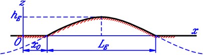
The case under consideration which is presented below concerns with the road excitation as a single pulse in which the road profile is a half cycle of sinusoidal wave. This type of road profile is described in Fig. 4 where $h_{E}$ and $L_{E}$ are respectively the height and length of the pulse. The values of $h_{E}$ and $L_{E}$ are taken as $h_{E} =$ 0.12 m, $L_{E} =$ 0.65 m. The distance $x_{0}$ in Fig. 4 is introduced for the generality of consideration and the clarity of graphs in time domain. The value of $x_{0}$ is calculated in accordance with a specified value of time ( $t_{0}$ ) and vehicle velocity ( $V$ ) by using the formula $x_{0} = V t_{0}$ (the value $t_{0} =$ 0.5 s is fixed in this paper).

Fig. 4Geometrical description of a half cycle of sinusoidal wave

Vibration of the vehicle will be considered in four different cases which involve the fact of taking road deformation (RD) and wheel separation (WS) into account or not. For ease of presentation, the four cases are denoted as follows:

Case 1: Taking account of both road deformation and wheel separation.

Case 2: Taking account of road deformation and ignoring wheel separation.

Case 3: Ignoring road deformation and taking account of wheel separation.

Case 4: Ignoring both road deformation and wheel separation.

3.1. Comparison of the results obtained from four consideration cases.

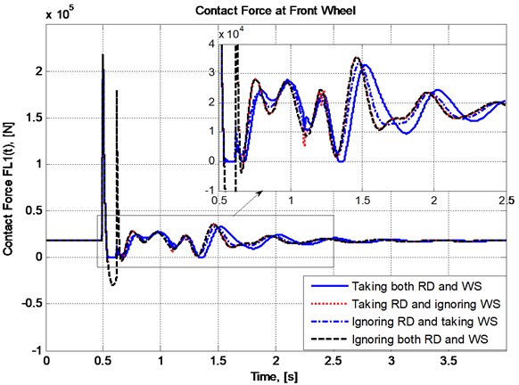
The plots in Fig. 5 and Fig. 6 present the changes in vertical displacement and acceleration of vehicle body while the plots in Fig. 7 and Fig. 8 respectively show the variation of contact forces at the front and the rear wheels with respect to time when the vehicle speed is taken as 20 km/h.

It can be seen from the plot form show that:

– Wheel separation really appear in the case of consideration. In Fig. 5, the plot of $u_{b} (t)$ has some pieces lying upper than zero level, and in Fig. 7 and Fig. 8, the plots of $F_{L 1} (t)$ and $F_{L 2} (t)$ in case 1 and case 3 have some flat pieces lying right on the abscissa.

– The plots in two cases of taking wheel separation into account (case 1 and case 3) have evident differences both in comparison with each other and with the other two cases.

– The differences in vertical displacements and accelerations between the two cases of disregarding wheel separation into account (case 2 and case 4) are not as significant as the differences in the same quantities between any other two cases. This means the effect of wheel separation on vehicle vibration is more significant than road deformation, and moreover, wheel separation makes the effect of road deformation become more significant at least in the situation of consideration.

Fig. 5The change in vertical displacement of vehicle body

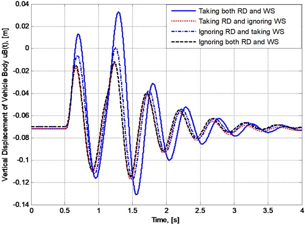
Fig. 6The change in vertical acceleration of vehicle body

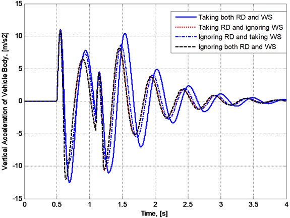
Fig. 7Variation of contact force at the front wheel

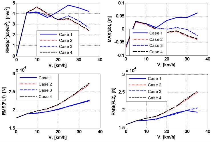
3.2. Effect of vehicle speed on response of the system

Table 1 presents some numerical results which reflect the effect of vehicle speed ( $V$ ) on the root mean square values RMS(.) of vertical acceleration of vehicle body and contact forces at the two wheels; the maximum value of vertical displacement of vehicle body. The used values of vehicle speed are discretely taken from 0 to 35 km/h. The graphs which depict the mentioned results are describe in Fig. 9. The results also involve the four considered cases mentioned above. The first column correspond to the static state of the vehicle ( $V =$ 0).

The plots in Fig. 9 show that:

– There are significant differences between the two cases of taking wheel separation into account in comparison with the two cases of disregarding this phenomenon. Especially, the difference in results between the two cases of not taking the loss of contact into account is not as much as the differences between any other two cases.

– The increase in vehicle speed leads to the increase in the RMS values of contact forces in general. The fact may involve the transformation of kinematic energy into potential energy of deformable parts.

– The effect of the increase in vehicle speed on the two other quantities (the RMS value of vertical acceleration and the maximum value of vertical displacement of vehicle body) does not follow an obvious trend. This may concerns the complexity in relations of geometrical parameters of the vehicle and the road profile and the velocity of movement.

– The RMS values of contact forces in the two cases of taking wheel separation into account are less than the corresponding values of the other two cases. This is reasonable because in periods of losing contact at any wheel, the contact force is equal to zero.

Fig. 8Variation of contact force at the rear wheel

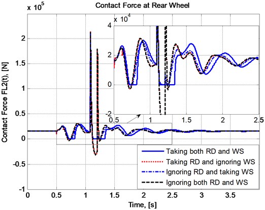
Table 1Effect of vehicle speed on RMS values of some typical quantities and the total time of losing contact

Vehicle speed (V), [km/h]		0	5	10	15	20	25	30	35
RMS ( ${\ddot{u}}_{b}$ ), [m/s²]	Case 1	0	4.0779	4.1048	3.6398	4.2111	4.7999	4.5314	4.1904
	Case 2	0	4.0779	4.5836	3.9364	3.3969	3.4797	2.9569	2.3620
	Case 3	0	4.1153	4.1521	3.8054	3.4496	3.8003	3.3325	2.6553
	Case 4	0	4.1153	4.6327	4.0155	3.4103	3.5263	3.0045	2.3996
RMS ( $F_{L 1}$ ), [N]	Case 1	17835	18869	19117	19514	20177	21056	21821	22654
	Case 2	17835	18869	19702	20301	21410	23123	25106	27101
	Case 3	17835	18889	19157	19560	20092	20971	21798	22542
	Case 4	17835	18889	19741	20373	21505	23280	25340	27427
RMS ( $F_{L 2}$ ), [N]	Case 1	15912	16882	17144	17526	18362	19241	19806	19338
	Case 2	15912	16882	17679	18170	19532	21107	23057	24977
	Case 3	15912	16904	17133	17373	18223	19009	19894	20623
	Case 4	15912	16904	17702	18234	19621	21254	23267	25266
$z_{b m a x}$ , [m]	Case 1	–0.0721	0.0284	0.0213	0.0067	0.0328	0.0445	0.0451	0.0621
	Case 2	–0.0721	0.0284	0.0180	–0.0025	–0.0133	–0.0093	–0.0264	–0.0392
	Case 3	–0.0702	0.0302	0.0202	0.0056	0.0006	0.0066	–0.0010	–0.0236
	Case 4	–0.0702	0.0302	0.0201	–0.0004	–0.0121	–0.0069	–0.0238	–0.0372

Fig. 9Effect of vehicle speed on RMS or maximum value of some parameters reflecting vibration of the vehicle

4. Conclusions

The article has made a longitudinal vibration model of a two-axle automobile where both road deformation and the loss of contact are taken into account. The automobile is modeled as a linear vibration system which has three masses and four degrees of freedom. The deformed road is modeled as an elastic beam which is simply supported at the two ends and lies on the Kelvin's visco-elastic ground. The model of wheel-road contact has taken account of wheel separation and the change in dimmension of the contact area if exists. The original differential equations of motion of the vehicle-road coupled system with a partial differential equation have been transformed into a system of all ordinary differential equations by applying the Bubnov-Galerkin’s method. An example of numerical computation has been fulfilled where the results of four different cases of formulation have been put in comparison and the effect of vehicle speed on vibration of the system has been considered. The obtained results proves the necessity of taking the loss of contact into account when considering vibration of vehicles.

References

Bala Raju A., Venkatachalam R. Analysis of vibrations of automobile suspension system using full-car model. International Journal of Scientific and Engineering Research, Vol. 4, Issue 9, 2013, p. 2105-2111.

Search CrossRef
Dung Nguyen D. Research on Dynamic Interaction in Vertical Direction between Automobiles and Roads. Ph.D. Thesis, Hanoi, Vietnam, 2018.

Search CrossRef
Gao W., Zhang N., Du H. P. A half-car model for dynamic analysis of vehicles with random parameters. Proceedings of the Fifth Australasian Congress on Applied Mechanics (ACAM 2007), Brisbane Australia, Vol. 1, 2007, p. 595-600.

Search CrossRef
Hu D., Yan Y., Liqun C., Shaopu Y. Vibration of vehicle - pavement coupled system based on a nonlinear foundation. Journal of Sound and Vibration, Vol. 333, Issue 24, 2014, p. 6623-6636.

Publisher
Jazar Reza N. Vehicle Dynamics-Theory and Application. Second Edition, Springer-Verlag New York, USA, 2014.

Search CrossRef
Lap Duc V. Vibration of Automobiles. People’s Army Publisher, Vietnam, 2011.

Search CrossRef
Mahmoud R., Atanu B. Passive suspension modelling and analysis of a full-car model. International Journal of Advanced Science Engineering Technology, Vol. 3, Issue 2, 2013, p. 250-261.

Search CrossRef
Mitra A., Benerjee N., Khalane H. A., Sonawane M. A., Joshi D. R., Bagul G. R. Simulation and analysis of full car model for various road profile on an analytically validated MATLAB/SIMULINK model. IOSR Journal of Mechanical and Civil Engineering (IOSR-JMCE), 2013, p. 22-33.

Search CrossRef
Mohd Azman A., Jazli Firdaus J., Ahmed E. M. Vehicle dynamics-modeling and simulation. first edition, centre for advanced research on energy. Technical University of Malaysia Malacca, 2016.

Search CrossRef
Spinola Roberto B. Vehicle Vibration response subjected to long wave measured pavement irregularity. Journal of Mechanical Engineering and Automation, Vol. 2, Issue 2, 2012, p. 17-24.

Publisher
Shaopu Y., Liqun C., Shaohua L. Dynamics of Vehicle-Road Coupled Systems. First Edition, Springer-Verlag Berlin Heidelberg, 2015.

Search CrossRef
Saopu Y., Saohua L., Yongjie L. Investigation on dynamical interaction between a heavy vehicle and road pavement. Vehicle System Dynamics. International Journal of Vehicle Mechanics and Mobility, Vol. 48, Issue 8, 2010, p. 923-944.

Publisher
Syabillah S., Samin P. M., Jamaluddin H., Rahman R. A., Burhaumudin M. S. Modelling and Validation of 7-DOF Ride Model for Heavy Vehicle. Proceedings of the International Conference on Automotive, Mechanical and Materials Engineering, 2012, p. 108-112.

Search CrossRef
Ham V. C., Dung N. D. Consideration on the loss of contact between the wheels of automobile and road surface caused by vertical vibrations. Proceedings of the National Conference on Engineering Mechanics, Danang Vietnam, Vol. 2, 2015, p. 108-115.

Search CrossRef
Cuong P. M., Dung T. Q., Nam L. H. Consideration on vibration of automobiles in quarter model with the loss of contact taken into account. Journal of Science and Technology, Military Technical Academy, Vietnam, Vol. 183, 2017, p. 64-73.

Search CrossRef
Ham V. C., Cuong P. M., Dung T. Q. Consideration of the problem about vibration of automobiles in one fourth model with taking road deformation and the loss of contact into account. Journal of Vibroengineering, Vol. 22, Issue 4, 2020, p. 945-958.

Publisher
Ham V. C., Cuong P. M., Dung T. Q. Consideration on vibration of automobiles in planar model taking account of the loss of contact. Proceedings of the National Conference on Mechanics and Transportation Engineering, Vol. 2, 2017, p. 236-332.

Search CrossRef
Dao Van D. Analysis on Stability and Dynamics of Structures made of Functionally Graded Materials. Publisher of Sciences and Engineerings, Vietnam, 2016.

Search CrossRef
Lap V. D. Handbook for looking up Specifications of Automobiles. Military Technical Academy, Vietnam.

Search CrossRef

About this article

Received

03 July 2020

Accepted

14 January 2021

Published

22 January 2021

SUBJECTS

Vibration in transportation engineering

DOI

https://doi.org/10.21595/jve.2021.21575

Keywords

vibration

automobile

planar model

half-car model

wheel separation

loss of contact

road deformation

This is an open access article distributed under the Creative Commons Attribution License, which permits unrestricted use, distribution, and reproduction in any medium, provided the original work is properly cited.

Previous article in issue Previous Next article in issue Next

Research article

2021 01 16

Consideration on lateral vibration of automobiles in quasi-planar model with wheel separation and road deformation taken into account

Ham Vu Cong, Cuong Phung Manh, Dung Tran Quang

Research article

2020 06 30

Consideration of the problem about vibration of automobile in one fourth model with taking road deformation and the loss of contact into account

Ham Vu Cong, Cuong Phung Manh, Dung Tran Quang

Research article

2018 12 31

Simplified theoretical treatment of lateral structural properties under crowd excitation

Yun Dong, Yan An Gao, Ye Zhu, Peng Zhang

Research article

2016 12 08

Determination of limit vehicle bump height in dynamic detection of simply supported bridge

Guojin Tan, Ziyu Liu, Yubo Jiao, Wensheng Wang

H. Vu Cong, C. Phung Manh, and D. Tran Quang, “Consideration of longitudinal vibration of automobiles in planar model with taking road deformation and loss of contact into account,” Journal of Vibroengineering, Vol. 23, No. 4, pp. 994–1010, Jan. 2021, https://doi.org/10.21595/jve.2021.21575

Copy Extrica

Copied to clipboard!

TY  - JOUR
DO  - 10.21595/jve.2021.21575
UR  - https://doi.org/10.21595/jve.2021.21575
TI  - Consideration of longitudinal vibration of automobiles in planar model with taking road deformation and loss of contact into account
T2  - Journal of Vibroengineering
AU  - Phung Manh, Cuong
AU  - Vu Cong, Ham
AU  - Tran Quang, Dung
PY  - 2021
DA  - 2021/01/22
PB  - JVE International Ltd.
SN  - 1392-8716
SN  - 2538-8460
ER  - 

Copy Ris

Copied to clipboard!

@article{Phung_Manh_2021,
	doi = {10.21595/jve.2021.21575},
	url = {https://doi.org/10.21595/jve.2021.21575},
	year = 2021,
	month = {jan},
	publisher = {{JVE} International Ltd.},
	author = {Cuong Phung Manh and Ham Vu Cong and Dung Tran Quang},
	title = {Consideration of longitudinal vibration of automobiles in planar model with taking road deformation and loss of contact into account},
	journal = {Journal of Vibroengineering}
}

Copy Bibtex

Copied to clipboard!

[1]C. Phung Manh, H. Vu Cong, and D. Tran Quang, “Consideration of longitudinal vibration of automobiles in planar model with taking road deformation and loss of contact into account,” Journal of Vibroengineering, Jan. 2021, doi: 10.21595/jve.2021.21575.

Copy IEEE

Copied to clipboard!

Phung Manh, Cuong, Ham Vu Cong, and Dung Tran Quang. “Consideration of Longitudinal Vibration of Automobiles in Planar Model with Taking Road Deformation and Loss of Contact into Account.” Journal of Vibroengineering, January 22, 2021. https://doi.org/10.21595/jve.2021.21575.

Copy Chicago

Copied to clipboard!

Consideration of longitudinal vibration of automobiles in planar model with taking road deformation and loss of contact into account

Abstract

Highlights

1. Introduction

2. Formulation of the problem

2.1. Assumptions

2.2. Contact characteristics between the wheel and the road

2.3. Vibration model of the vehicle-road coupled system

2.4. Determination of forces acting on the automobile

2.5. Differential equations of motion of the mechanical system

2.5.1. Differential equations of motion of the vehicle

2.5.2. Differential equation of motion of the deformed road

2.6. Simpler particular cases of the differential equations of motion

2.6.1. The case of ignoring road deformation

2.6.2. The case of disregarding the loss of contact

2.6.3. The case of ignoring both the road deformation and the loss of contact

2.7. Transforming the differential equations of motion into a system of all ODEs

2.8. Initial conditions

3. Some results from numerical computation

3.1. Comparison of the results obtained from four consideration cases.

3.2. Effect of vehicle speed on response of the system

4. Conclusions

References

About this article

Related Articles