Study on flow dynamic characteristic of bladder pressure pulsation attenuator based on dynamic mesh technology

Xin, Qing; Zhang, Yongxiang; Li, Jiawei

doi:10.21595/jve.2021.21725

Journal of Vibroengineering

Browse Journal

Submit article

Published: 11 February 2021

Check for updates

Study on flow dynamic characteristic of bladder pressure pulsation attenuator based on dynamic mesh technology

Qing Xin¹

Yongxiang Zhang²

Jiawei Li³

^{1, 2, 3}College of Power Engineering, Naval University of Engineering, Wuhan, China

Corresponding Author:

Yongxiang Zhang

Cite the article Download PDF

Downloads 934

Abstract

To solve the problem that the flow dynamic characteristic of the bladder pressure pulsation attenuator cannot be quantitatively analyzed, a bladder pressure pulsation attenuator was taken as the research object, and the dynamic mesh technology was combined with the User-Defined-Function (UDF) to numerically simulate the working process of the attenuator. Overcoming the divergence problem in finite-element fluid calculation and the negative volume problem in mesh updating process, the bladder pressure pulsation attenuator was dynamically simulated under different fluctuating frequencies and different inflatable pressure, the change of internal flow field was monitored in time. The results show that the resistance loss through the attenuator increases with the increase of the frequency and the increase of the charging pressure. The local resistance loss is much higher than the frictional resistance loss. The simulation results match the experimental results, that verifies the model's validity and correctness, and also provides a new method and idea to improve bladder attenuator's resistance loss and analyze the variable boundary problem.

Study on flow dynamic characteristic of bladder pressure pulsation attenuator based on dynamic mesh technology

Highlights

The dynamic mesh technology was combined with the User-Defined-Function (UDF) to numerically simulate the working process of the attenuator.
The flow rate of screw pump increases, the flow rate of lubricating oil inside the attenuator increases, and the resistance loss of the bladder attenuator increases.
Providing a new method and idea to improve bladder attenuator's resistance loss and analyze the variable boundary problem.

1. Introduction

A piping system may become a severe hidden problem of engineering safety since its service life and operational accuracy could be affected by the vibration resulting from the pulsation of flow rate and pressure. Installing a pulsation attenuator in the pipeline system is the most widely used method for attenuating pressure pulsation and reducing fluid noise [1, 2].

To satisfy the needs of engineering, attenuator has been extensively studied at home and abroad. The acoustic performance, hydrodynamic performance and structural performance of the attenuator are the focus of research. As early as 1871, Baldwin began to study the energy storage pressure fluctuation attenuator and applied for a patent [3]. KenIchirgu simplified the bladder movement of the bladder attenuator. He started to change the cross-sectional area of the bladder in contact with the oil to change the attenuator’s research on high-frequency pulsation suppression through experiments [4, 5]. Japanese scholars put forward an insertion loss characteristic expression for attenuator from the acoustic perspective, and determined the optimal position for inserting attenuator in a theoretical way, so as to help effectively find the optimal position for insertion [6]. Wang et al. deduced the insertion loss of bladder-type attenuator by virtue of transfer matrix [7], but insertion loss could not reflect the pulsation attenuation characteristics in front of and behind attenuator, and not be used to analyze the influence of the structural dimensions of attenuator on its attenuation properties. Reference [8] simplified the attenuator to a gas spring-damping model, and established a mathematical model of the bladder attenuator. Reference [9] adopted the same mathematical model theory to analyze and obtained the optimal attenuation effect of the attenuator when the operating frequency is the same as the natural frequency. However, this model cannot fully explain the influence of the structural parameters of the bladder and the attenuator on the performance of the attenuator. Reference [10] proposed a pipeline pressure pulsation suppression device based on the principle of damper and orifice plate filtering, using attenuator group to suppress low-frequency pressure pulsation and orifice plate to suppress high-frequency pressure pulsation. The test showed that the attenuation reached up to 50 % when the flow rate was pulsed at 20 Hz, but this study did not carry out an in-depth theoretical analysis of the attenuator group, and there was a disadvantage of large volume. Luo et al. presented a calculation method for optimizing multiple accumulators. Simulation and experiment analyses revealed that integrating multiple accumulators into a seawater piston pump and optimizing the precharged parameters can reduce the pressure pulsation under different levels of working back pressure [11]. Kumar et al. studied the control of pressure fluctuation in a hydraulic system and the energy savings from fluctuation by using a bladder-type hydraulic accumulator. A simulation of the hydraulic system was conducted on MATLAB/Simulink. The results showed that the ability to absorb fluctuation and stabilize the system is high in a small capacity accumulator. A time lag occurs as the size of the accumulator increases [12]. Zhao et al. designed a new type of double-bladder attenuator, and analyzed the relationship between its natural frequency and structural parameters based on a Maxwell mechanical model, so as to provide a new approach to the analysis of duplex attenuator characteristics [13]. Reference [14] simplified the mechanical model of the bladder-type attenuator, provided theoretical support for the better selection of the initial volume and pre-inflation pressure of the attenuator through programming simulation and in-depth analysis of the performance of the attenuator. Based on the above mechanical model, Li Mingjie et al. used AMESim software to carry out simulation analysis on the bladder attenuator. The system pressure impact was relatively low when the pre-inflated pressure of the attenuator was 80 % ~ 90 % of the working pressure of the system [15]. Nevertheless, their studies only focused on the static effect of fixed fluid pressure, and overlooked the coupling effect of fluid and bladder when the pulsating fluid flows through the attenuator.

In the previous studies on the acoustic performance, hydrodynamic performance and structural performance of the bladder attenuator, the coupling effect of the bladder and the pressure oil has been ignored, and the problem of the bladder variable boundary has been simplified into a fixed boundary problem for analysis. Therefore, the performance of the balloon attenuator could not be analyzed in a real way. Because the bladder attenuator exchanges energy through the bladder boundary during operation, the boundary shrinks and expands continuously, its calculation boundary changes constantly, and the internal flow field is constantly changing. It is a typical nonlinear and unsteady fluid problem with variable boundary. Classical methods are often difficult to obtain analytical results, and theoretical models are difficult to quantify the performance of attenuators, and cannot meet the fine analysis required by modern industry. With the development of finite element calculation software, there have been many successful cases of using dynamic mesh technology to study the problem of variable boundaries. For example, Reference [16] used dynamic grid technology to successfully predict the growth of dynamic cracks. The model proposed in the article is very suitable for predicting the material discontinuities commonly observed in composite structures. Reference [17] used dynamic grid technology to perform CFD analysis on the wing's static and time-varying deformation, and developed an unsteady transient analysis method for deformed airfoils. Reference [18] studied the mechanism of steam flow excited vibration and its influence on the dynamic characteristics of the rotor based on the mesh deformation simulation of the rotation motion of the three-dimensional rotor. Reference [19] established a CFD finite element model based on the erosion-dynamic mesh coupling theory, and analyzed the impact of sand on the erosion evolution of the wire-wound screen during the sand control process. Reference [20] introduced VOF multiphase flow model and Schnerr-SAUer cavitation model based on the finite volume method of N-S equation. Combined with the dynamic grid technology, the numerical calculation models of underwater two-lien projectiles and three-lien projectiles were established respectively, and the resistance characteristic curves of the projectiles were obtained. In reference [21], in order to analyze the characteristics of the cavitation flow field of a non-concentric squeeze film damper, a three-dimensional numerical model of unsteady cavitation flow field was built by using the mixture multiphase flow model and the moving grid technology, and the pressure and gas phase volume fraction distribution of the flow field of the squeeze oil film damper at different moments of the inner ring inculcations under different oil supply pressures were calculated. It can be seen from the above successful cases that the dynamic grid technology can be used to solve the problem of variable boundaries. Combined with the dynamic grid technology, a numerical analysis model based on CFD is established according to the features of bladder pulsation attenuator, so as to analyze the relationship between the performance and structure of pulsation attenuator, optimize the structure of attenuator, and improve the work performance of attenuator in a comprehensive way. This will lead the study of pulsation attenuation into a new field.

In order to accurately predict the fluid dynamic characteristics of the attenuator, this paper establishes the mathematical model and three-dimensional model of the bladder pressure pulsation attenuator. The dynamic mesh technology was combined with user-defined functions (UDF) to simulate the bladder movement and perform the numerical calculation. The flow field inside the attenuator is monitored in time, the resistance loss of the bladder attenuator in the working process is calculated, the factors affecting the resistance loss and the law of influence are analyzed, and a test bench is built for experimental verification.

2. The mechanism of bladder attenuator resistance loss

The acoustic performance, hydrodynamic performance and structural performance of the bladder attenuator are interrelated and mutually restricted, so the research on the hydrodynamic performance of the attenuator is very important. According to the mechanism of resistance loss, resistance loss can be divided into two categories [22]: friction resistance loss and local resistance loss.

2.1. Friction resistance loss

The frictional resistance of the fluid is caused by the viscosity that appears when the fluid moves. The frictional resistance can be calculated according to the Darcy-Weisbach formula as follows:

1

V p = λ \frac{l}{d} \frac{ρ v_{0}^{2}}{2} .

Among them, $l$ and $d$ are the equivalent length and diameter of the attenuator, $ρ$ is the fluid density, $v_{0}$ is the fluid velocity, and $λ$ is the coefficient related to the Reynolds number of the fluid flow.

2.2. Local resistance loss

The local resistance loss of the fluid is produced when the normal flow is locally damaged. When the fluid flows pass through the attenuator, the fluid diffuses, shrinks, bends and branches. The rate, direction of the fluid flow or both of them change, causing the partial fluid to exchange momentum and vortex, thus consuming energy and producing a local pressure drop, which is called local drag loss. The calculation formula of local resistance loss is as follows:

2

∆ p = ξ \frac{ρ v_{0}^{2}}{2} .

Among them, $ξ$ is called the local drag coefficient, which depends on the local change of the attenuator structure.

The cross-section of the connection between the attenuator and the pipeline changes greatly, and the local resistance loss when the fluid flows through the attenuator is much greater than the frictional resistance loss. The resistance loss studied in this paper is the total resistance loss, which is calculated by the formula $∆ p = p_{1} - p_{2}$ (where: $p_{1}$ is the inlet pressure of the attenuator and $p_{2}$ is the outlet pressure of the attenuator).

3. Simulation analysis of bladder attenuator

3.1. Physical model of bladder attenuator

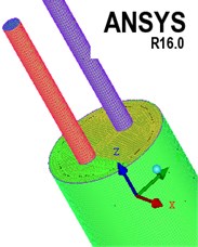
The structure diagram of the bladder attenuator is presented in Fig. 1. The main dimensions of the attenuator are: bladder $V =$ 25 $L$ , $L_{1} =$ 918.5 mm, $d_{1} =$ 280 mm, $d_{2} =$ 42 mm. When the fluid flows through the attenuator, the pressure of the fluid causes the bladder to deform. The three-dimensional method is used to simulate the resistance loss of the attenuator. The key issue is the correct handling of the bladder movement. The bladder attenuator in this article does not consider the elastic modulus of the bladder when building the model, and treats the bladder as a rigid wall. The movement of the bladder is transformed into a “gas spring-damper model”. The physical model of the attenuator is presented in Fig. 2.

Fig. 1Structure diagram of bladder pressure pulsation attenuator

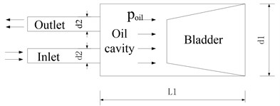
Fig. 2Simplified model of bladder pressure pulsation attenuator

3.2. Calculation model of bladder attenuator

In this paper, the flow velocity of the fluid is much lower than the sound velocity of 1480 m/s in water, and the density change of the fluid can be ignored, which is regarded as an incompressible flow. This article studies the unsteady turbulent motion. It is generally believed that no matter how complicated the turbulent motion is, the unsteady continuous equation and Navier-Stokes equation are applicable to the instantaneous motion of turbulence. The components of the velocity vector $u$ in the $x$ , $y$ , and $z$ directions are $u$ , $v$ , and $w$ , and the instantaneous turbulent control equations are as follows [23]:

3

d i v u = 0,

4

\frac{\partial u}{\partial t} + d i v (u u) = - \frac{1}{ρ} \frac{\partial p}{\partial x} + v d i v (g r a d u),

5

\frac{\partial v}{\partial t} + d i v (v u) = - \frac{1}{ρ} \frac{\partial p}{\partial y} + v d i v (g r a d v),

6

\frac{\partial w}{\partial t} + d i v (w u) = - \frac{1}{ρ} \frac{\partial p}{\partial z} + v d i v (g r a d w) .

At present, the most widely used turbulence model for numerical simulation is the standard $k$ - $ε$ model. In the standard $k$ - $ε$ model, $k$ and $ε$ are two basic unknowns, and the corresponding transportation equation is as follows [24]:

7

\frac{\partial}{\partial t} (ρ k) + \frac{\partial}{\partial x_{i}} (ρ u_{j} k) = \frac{\partial}{\partial x_{j}} [(μ + \frac{μ_{t}}{σ_{k}}) \frac{\partial k}{\partial x_{j}}] + G_{k} + G_{b} - ρ ε - Y_{M} + S_{K},

8

\frac{\partial}{\partial t} (ρ ε) + \frac{\partial}{\partial x_{i}} (ρ ε u_{i}) = \frac{\partial}{\partial x_{j}} [(μ + \frac{μ_{t}}{σ_{ε}}) \frac{\partial ε}{\partial x_{j}}] + C_{1 ε} \frac{ε}{k} (G_{k} + C_{3 ε} G_{b}) - ρ C_{2 ε} \frac{ε^{2}}{k} + S_{ε} .

In these laws, $ρ$ is fluid density; $u$ , $v$ , $w$ are the velocity component of velocity vector in the directions $x$ , $y$ and $z$ ; $μ$ is dynamic viscosity of fluid; $μ t$ is turbulent viscosity; $f$ is traversing force; $G k$ , $G b$ are turbulent energy terms; $C_{1}$ , $C_{2}$ , $C_{3}$ are empirical constants, which are 1.44, 1.92, and 0.99 respectively; $σ k$ , $σ ε$ are Prandtl numbers of turbulence, which are 1.0 and 1.3 respectively.

3.3. Dynamic mesh technology

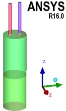
The calculation model of attenuator is cylindrical, so that there are very high requirements for the quality of mesh because of the generation and elimination of meshes in the motion of bladder. For this reason, structured mesh generation calculation model is adopted since it features good quality, simple data structure, and smooth area, and it is easier to approximate the actual model, so as to prevent the occurrence of negative volume as much as possible. For several different parts of the pipeline, oil cavity and bladder, different blocks are created respectively, and the parts are processed as O-Block. The local division and local mesh are shown in Fig. 3.

Fig. 3Schematic diagram of local subdivision and mesh

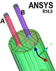
It can be seen from Figs. 1 and 2 that the movement of the bladder is affected by the combination of the oil cavity, the air pressure in the bladder, its own gravity and other forces. The oil pressure changes cause the bladder to move, which makes the air pressure change. The bladder movement is coupled with the flow field. It is difficult to express it in expressions. The coupling movement of the bladder and the flow field is described by writing a macro function. The movement area includes the movement of the bladder and the deformation of the cylindrical surface. The movement of the bladder is described by a user-defined function. Its core is the macro function DEFINE-SDOF-PROPERTIES. The principle of the macro function is to release the translational freedom of the $Z$ axis and constrain $X$ , $Y$ axis translation and $X$ , $Y$ , and $Z$ axis rotation (the positions of $X$ , $Y$ , and $Z$ are shown in Fig. 3, where the $Z$ axis is the axial direction of the attenuator); the cylindrical surface is used as the deformation area by setting the cylindrical surface deforming, the movement process is controlled by the cylinder. The mesh update method selects the dynamic layer method, the control parameter selects the constant height option, and the default split factor and merge factor are maintained.

3.4. Simulation scheme

The fluid medium is 46# lubricating oil with initial temperature 40 ℃, density 860 kg/m³ and kinematic viscosity 46 mm²/s. The boundary conditions are as follows:

(1) Wall boundary conditions.

The viscous fluid has no translation or rotation at the boundary of the wall, and the boundary condition of speed must satisfy the non-slip condition, so the wall is set as a non-slip wall.

(2) Inlet boundary conditions.

The power of the experiment in this article comes from the twin-head screw pump. In order to be unified with the subsequent experimental verification, the simulation inlet boundary is set as a pressure inlet with sinusoidal regular fluctuations to simulate different inlet conditions at the output of the screw pump. The inlet conditions are defined by a user-defined function (UDF) definition.

(3) Outlet boundary conditions.

The outlet boundary condition is set to static pressure outlet, and the outlet pressure is set to zero, which is easier to converge in the iterative calculation.

The main purpose of this simulation is to simulate and calculate the resistance loss when the fluid flows pass through the attenuator. It can be seen from formula 1 and 2 that the resistance loss is mainly affected by the structure of the attenuator and the fluid flow rate. By setting different speeds and inlet velocity, the resistance loss of the attenuator under different working conditions is simulated. In order to accurately measure the pressure, after the system is stabilized, the velocity vector diagram of the attenuator is observed to avoid the fluid backflow area and the measuring points A and B are arranged as shown in Fig. 3.

Table 1Simulation conditions

Frequency $f$ / Hz	18	22	26	30	34	38	42	46
Rotate speed $r$ / min	540	660	780	900	1020	1140	1260	1380
Inlet velocity $m$ / s	0.62	0.77	0.91	1.05	1.19	1.33	1.48	1.61

This paper takes a self-made pressure pulsation attenuator as the research object. According to the actual working conditions, the average pressure of the system is selected as 0.8×10⁶Pa, and the initial inflation pressure of the bladder is 0.2×10⁶Pa-0.5×10⁶Pa. The flow process in the pipeline and attenuator is considered to be adiabatic, without considering the energy exchange with the outside world. According to the theoretical flow calculation formula of screw pump [25] $Q = 2 A T n$ ( $Q$ is the flow, $A$ is the cross sectional area of the spiral working length, $T$ is the spiral lead, and n is the rotate speed), the inlet velocity at different speeds can be calculated. The simulation operating conditions are set as shown in Table 1.

3.5. Mesh number independence test

For non-steady-state numerical simulations, it is necessary to determine the mesh independence verification between the number of meshes used and the results of the calculation. This paper studies the resistance loss caused by fluid flowing through the attenuator, so the pressure value in the simulation calculation results needs to be independently tested. When the bladder pressure is 0.5×10⁶Pa and the pulse frequency of the lubricant is 18 Hz, the five different mesh quantities are independently tested, and the average result of the pressure of inlet A and outlet B is obtained when the system pressure stabilizes, as shown in Table 2.

As can be found from Table 2, the number of meshes has a great impact on the simulation results, when the number of meshes is less than 270,000, the simulation results vary greatly, and when the number of meshes is greater than 270,000, the simulation results tend to stabilize. Taking into account the simulation time and simulation error, it is concluded that the independence requirements of the number of grids can be met when the number of grids is 277370.

Table 2Results of mesh number independence test

Content	Mesh quantities
Content	131885	190752	277370	426576	739047
Average inlet pressure / Pa	854156	865632	795482	793588	794215
Average outlet pressure / Pa	815475	826588	731268	730025	730894

3.6. Simulation results and analysis

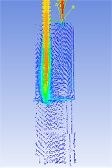
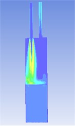
Fig. 4 is the velocity vector diagram and turbulent kinetic energy clouds when the bladder pressure is 0.5×10⁶Pa and the lubricating oil pulsation frequency is 18 Hz and the system pressure is stable. It can be seen from the figure that when the fluid flows into the attenuator, at the entrance of the attenuator, part of the fluid maintains its original state of motion, while the other part quickly spreads to the attenuator, and has irregular motions such as vortices and vortices, and the fluid collides on the wall surface, the size and direction of the fluid velocity have changed at this time, resulting in energy loss. After the fluid enters the attenuator, it contacts the bladder, causing resistance loss again. Finally, a similar fluid phenomenon occurs again when the fluid flows out of the attenuator, a resistance loss occurs. Therefore, the fluid flow state changes when the fluid flows through the attenuator, causing resistance loss.

Fig. 4Velocity vector graphs and turbulent kinetic energy clouds

When the bladder pressure is 0.5×10⁶Pa and the lubricating oil pulsation frequency is 18 Hz, according to the simulated pressure response curve in Fig. 5, the analysis shows that when the system pressure is stable, the maximum pressure at the inlet is 836×10³Pa, the minimum pressure is 755×10³Pa and the average pressure is 795.5×10³Pa. The maximum pressure at the outlet is 758×10³Pa, the minimum pressure is 704×10³Pa, and the average pressure is 731×10³Pa. At this point, the resistance loss is 64.5×10³Pa. Similarly, when the bladder pressure is 0.5×10⁶Pa and the lubricating oil pulsation frequency is 46 Hz, according to the simulated pressure response curve in Fig. 6, the analysis shows that when the system pressure is stable, the maximum pressure at the inlet is 867×10³Pa, the minimum pressure is 730×10³Pa and the average pressure is 798.5×10³Pa. The maximum pressure at the outlet is 698×10³Pa, the minimum pressure is 658×10³Pa, and the average pressure is 678×10³Pa. At this point, the resistance loss is 120.5×10³Pa.

By using the same method to calculate and analyze other working conditions, the results of the resistance loss in other working conditions can be obtained. Table 3 shows the results of the resistance loss when the attenuator is simulated under different working conditions. It can be seen from the simulation results in Table 3 that the attenuator's resistance loss is different under different working conditions.

With the increase of the lubricating oil pulsation frequency, the resistance loss when the fluid flows through the attenuator continues to increase. The reason is that the speed of the screw pump increases, which increases the lubricating oil pulsation frequency, causing the increase in the flow rate of the screw pump and making the lubricating oil in the attenuator the flow rate increases continuously, which in turn increases the resistance loss, and the simulation results conform to the theoretical calculation rules of Literature 22. With the increase of the inflation pressure of the bladder, the resistance loss of the fluid flowing through the attenuator increases continuously. The reason is that after the increase of the initial aeration pressure of the bladder, the volume of the bladder becomes larger, and the contact area between the oil and the bladder becomes larger, which makes the resistance loss becomes larger.

Fig. 5Simulation pressure response curve when the bladder pressure is 0.5×106 Pa and 18 Hz

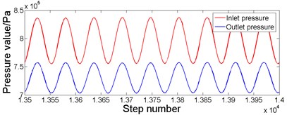
Fig. 6Simulation pressure response curve when the bladder pressure is 0.5×106 Pa and 46 Hz

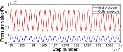
Table 3Resistance loss ∆P / 103 Pa simulation results

Bladder pressure $p_{0}$ / 10⁶Pa	Frequency $f$ / Hz
Bladder pressure $p_{0}$ / 10⁶Pa	18	22	26	30	34	38	42	46
0.2	50	59	61	68	75	84	92	98
0.3	55	67	72	75.5	81	90	98	106
0.4	62	70.5	81	87	90	95	105	111
0.5	64.5	71	82	90	94	98	109	120.5

4. Experimental study

4.1. Experimental principle and scheme

In order to verify the correctness and feasibility of the dynamic grid technology for calculating the resistance loss of the attenuator, an experimental platform was built according to the actual layout of a certain type of diesel engine lubricating oil pipeline, and the experiment verified the actual engineering and simulation content. The experimental platform was mainly comprised of double-head screw pump, oil tank, lubricating oil pipeline, bladder-type attenuator, precision pressure gauge, and control box, and its schematic diagram and facilities are as shown in Fig. 7 and Fig. 8. Due to the long pipeline, in order to accurately obtain the pressure value of the inlet and outlet of the attenuator, select the position close to the gate valve 1 and 2 to set the measuring points 1 and 2, and compare the data by selecting the same working conditions as the simulation to verify the reliability of the simulation. When the test bench is working, the gate valves 1 and 2 are opened. At this time, the lubricating oil is output from the screw pump, passes through the attenuator, and returns to the oil tank from the throttle valve 3 through the circulation loop. The rotation speed of the screw pump is controlled by the control box, the pulsation frequency of the inlet lubricating oil is controlled, the throttle valve 3 is adjusted to make the oil circuit reach the required oil pressure. By analyzing and comparing the pressure of measuring points 1 and 2, the resistance loss of the pulsating oil pressure through the attenuator can be obtained.

Fig. 7Schematic diagram of attenuator resistance loss experiment

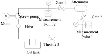
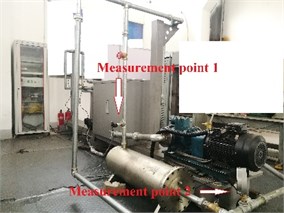
Fig. 8Attenuator resistance loss experiment platform

The same frequency and work pressure as used in simulation were selected for the experiment. The work pressure was set to 0.8×10⁶Pa. The main frequency of oil pulsation in the piping system was twice of the rotational frequency of double-head screw pump. The setting of operating conditions is presented in Table 4. The test system for the experiment was comprised of HM90-H2-3-V2-F1-W2 pressure sensors with the range of 0-3×10⁶Pa, B&K3610-A-042 data collector with the highest sampling frequency of 131,072Hz, and pressure gauges. The output end of pressure sensor was connected to the PLUSE system collector produced by B&K for transmission to computer. The signal sampling frequency in the experiment was 32,768 Hz.

Table 4Experimental conditions

Frequency $f$ / Hz	18	22	26	30	34	38	42	46
Rotate speed $r$ / min	540	660	780	900	1020	1140	1260	1380

Table 5Sensor calibration data

Output voltage / V		Pressure measurement / 10⁶×Pa
Measurement point 1	Measurement point 2	Pressure measurement / 10⁶×Pa
0.32	0.43	0.2
0.64	0.77	0.4
0.97	1.11	0.6
1.30	1.46	0.8

The range of HM90-H2-3-V2-F1-W2 pressure sensor is 0-3×10⁶Pa, the accuracy is 0.1 % and the signal output is 0-5 V. Due to the influence of region and time on the sensor for a long time in use, the sensor will drift to some extent. The manual calibration of the pressure sensor is carried out according to the method in Literature 26 to reduce the influence of measurement error on the experiment. Calibration parameters are shown in Table 5. After fitting the calibration parameters, the following linear relationship is obtained between the measured pressure values of sensor 1 and sensor 2 and the output voltage:

9

Y = 608640 X + 8295.3,

10

Y = 585470 X - 52459 .

In these laws, $X$ is output voltage and $Y$ is measured pressure.

4.2. Analysis of experimental results

Import the experimental data into MATLAB for filtering processing, and obtain the time-pressure curve around measuring points 1 and 2. When the bladder pressure is 0.5×10⁶Pa and the lubricating oil pulsation frequency is 18Hz, according to the experimental data in Fig. 9, the analysis shows that when the system pressure is stable, the maximum pressure at the inlet is 745×10³Pa, the minimum pressure is 716×10³Pa, and the average pressure is 731×10³Pa. The maximum pressure at the outlet is 663×10³Pa, the minimum pressure is 653×10³Pa, and the average pressure is 658×10³Pa. At this time, the resistance loss is 78×10³Pa. Similarly, when the bladder pressure is 0.5×10⁶Pa and the lubricating oil pulsation frequency is 46 Hz, according to the experimental data in Fig. 10, the analysis shows that when the system pressure is stable, the maximum pressure at the inlet is 817×10³Pa, the minimum pressure is 749×10³Pa, and the average pressure is 781×10³Pa. The maximum pressure at the outlet is 668×10³Pa, the minimum pressure is 643×10³Pa, and the average pressure is 654×10³Pa. At this time, the resistance loss is 127×10³Pa.

Fig. 9Experimental pressure response curve when the bladder pressure is 0.5×106Pa and 18 Hz

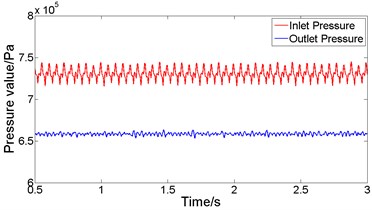
Fig. 10Experimental pressure response curve when the bladder pressure is 0.5×106Pa and 46 Hz

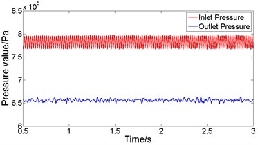
Table 6Resistance loss ∆P / 103 Pa experimental results

Bladder pressure $p_{0}$ / 10⁶Pa	Frequency $f$ / Hz
Bladder pressure $p_{0}$ / 10⁶Pa	18	22	26	30	34	38	42	46
0.2	59	66	69	76	84	91	101	111
0.3	63	72	83	87	92	100	110	115
0.4	69	79	87	91	100	108	115	120
0.5	73	80	89	93	103	109	116	127

Table 6 is the experimental results of the resistance loss when the attenuator is working under different working conditions. From the experimental results in Table 6, it can be found that with the increase of frequency, the resistance loss continues to increase, which is consistent with the simulation results, and this conforms to the law of theoretical analysis. As the inflation pressure of the bladder increases, the resistance loss continues to increase, which is consistent with the simulation results.

Fig. 11Simulation and experimental results at different frequencies at 0.2× 106Pa

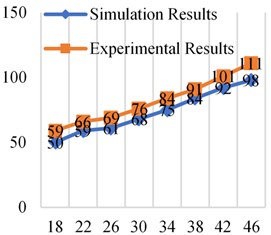
Fig. 12Simulation and experimental results at different frequencies at 0.3×106 Pa

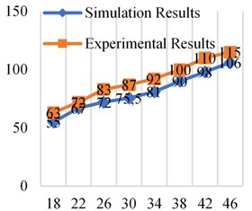
Fig. 13Simulation and experimental results at different frequencies at 0.4×106 Pa

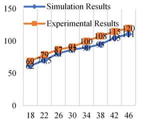
Fig. 14Simulation and experimental results at different frequencies at 0.5×106 Pa

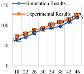
From the comparative analysis of the experimental results and simulation results in Figs. 11-14, it can be found that the experimental results are higher than the simulation results. The reasons include the following aspects. One is that the elastic model of the bladder is ignored in the simulation and simplified into a “gas spring-damping model”, which makes the contact area between the oil and the bladder smaller and makes the simulation value lower than the experimental value. Second, the simulation analysis did not take into account the friction between the fluid and the pipe wall and the inner surface of the attenuator. However, the inner surface of the bladder-type attenuator used in the experiment was not smooth enough and had burrs. Third, it can be seen from the design of the experimental platform that there are pipe joints and pressure gauges between measuring point 1 and measuring point 2. The setting of these fluid components will also have a certain impact on fluid resistance, which is not considered in the simulation analysis. In addition, there are errors in experimental measurements.

The error between the experimental results and the simulation results is within the acceptable range, so it is feasible and effective to use dynamic grid technology to simulate the bladder movement and analyze the resistance loss of the bladder attenuator in the working process.

5. Conclusions

In this paper, a numerical analysis model of the bladder attenuator is established based on the dynamic grid technology. The motion of the bladder is simulated numerically by combining the user-defined function, and the flow field inside the attenuator is analyzed. The following conclusions are obtained:

1) The resistance loss of the capsule attenuator consists of local resistance loss and frictional resistance loss, among which the local resistance loss is much larger than the frictional resistance loss.

2) Both simulations and experiments show that within a certain range, the initial inflation pressure of the bladder increases, the volume of the bladder continues to increase, and the resistance loss of the attenuator is also greater.

3) Both simulation and experiment show that with the increase of the speed of screw pump, the flow rate of screw pump increases, the flow rate of lubricating oil inside the attenuator increases, and the resistance loss of the bladder attenuator increases.

4) The simulation results are basically consistent with the experimental results, and the variation law of the resistance loss is consistent, which indicates that the simulation calculation method based on the dynamic grid technology is feasible and effective for the bladder attenuator, which provides a new idea for the correct prediction of the performance of the bladder attenuator, and also provides a new method for the study of the variable boundary problem.

References

Li H., Zhu Y., Xin Y. Modeling and simulation of a hydro-pneumatic accumulator system for hybrid air development. Applied Mechanics and Materials, Vol. 733, 2015, p. 763-767.

Publisher
Bao J., Cen Y., Ye X. Researches on the energy regeneration and vibration reduction performance of a new hydraulic energy regenerative suspension. Proceedings of the 6th International Asia Conference on Industrial Engineering and Management Innovation, 2014, p. 605-615.

Publisher
Baldwin J. S. Improvement in Accumulators for Liquids Under Pressure. US Patent, US121482, 1871.

Search CrossRef
Ichiryu K. Development of Accumulator for High Frequency Ripple Absorption. Bulletin of JSME, Vol. 15, Issue 88, 1972, p. 1215-1227.

Publisher
Ichiryu K. Vibration Damping Method of Hydraulic System by Accumulators. Bulletin of JSME, Vol. 12, Issue 53, 1969, p. 1110-1120.

Publisher
Eiichi K., Takayoshi I. Research on pulsation attenuation characteristics of silencer in real hydraulic systems. International Journal of Fluid Power, Vol. 1, Issue 2, 2000, p. 29-38.

Publisher
Xie P., Wang Q. Study on the effect of accumulator on reducing fluid pulsation in pipeline. Noise and Vibration Control, Vol. 2, 2000, p. 2-5, (in Chinese).

Search CrossRef
Quan L., Kong X., Gao Y. The shock absorption theory and experiment of accumulator without considering the import characteristics. Chinese Journal of Mechanical Engineering, Vol. 9, 2007, p. 28-32, (in Chinese).

Publisher
Li L., Wang H., Gong L. Parameter analysis and test of bladder accumulator to absorb pressure pulsation. Hydraulics and Pneumatics, Vol. 7, 2012, p. 3-6, (in Chinese).

Search CrossRef
Zhao D., Luo X., Yang Z. Optimal design and test analysis of a pipeline pressure pulsation suppression device. Noise and Vibration Control, Vol. 6, 2014, p. 188-191, (in Chinese).

Search CrossRef
Luo X., Cao Sh., Shi W. Analysis and design of a water pump with accumulators absorbing pressure pulsation in high-velocity water-jet propulsion system. Journal of Marine Science and Technology, Vol. 20, Issue 3, 2015, p. 551-558.

Publisher
Kumar A., Das J., Barnwal Dasgupta K. Effect of hydraulic accumulator on pressure surge of a hydrostatic transmission system. Journal of the Institution of Engineers (India): Series C (Mechanical, Production, Aerospace and Marine Engineering), Vol. 99, Issue 2, 2018, p. 169-174.

Publisher
Zhao W., Ye Q. Thermodynamic system analysis of a new compound skin accumulator. Journal of System Simulation, Vol. 12, 2017, p. 3149-3159, (in Chinese).

Search CrossRef
Dong M., Luan X., Liang J. Analysis of dynamic characteristics of bladder-type accumulator to absorb pulsation. Hydraulics and Pneumatics, Vol. 5, 2019, p. 109-116, (in Chinese).

Search CrossRef
Li M., Wu Zh., Xu G. Simulation and experimental research on the influence of main parameters of accumulator on hydraulic vibration platform system. Hydraulics and Pneumatics, Vol. 9, 2019, p. 70-77, (in Chinese).

Search CrossRef
Francesco F., Marco F. F., Fabrizio G. Dynamic crack growth based on moving mesh method. Composites: Part B, Engineering, Vol. 174, 2019, p. 107053.

Publisher
Chawki Abdessemed, Yufeng Yao, Abdessalem Bouferrouk, et al. Morphing airfoils analysis using dynamic meshing. International Journal of Numerical Methods for Heat and Fluid Flow, Vol. 28, Issue 5, 2018, p. 1117-1133.

Publisher
Si H., Cao L., Li P. Dynamic characteristics and stability prediction of steam turbine rotor based on mesh deformation. Energy and Ecology, Vol. 66, Issue 3, 2020, p. 164-174.

Publisher
Sun Yan, Lou Yishan, Cao Yanfeng, et al. Numerical simulation of the erosion process of the wire-wrapped screen based on the erosion-dynamic grid coupling. Petroleum Drilling and Production Technology, 2020.

Search CrossRef
Shi H., Zhou D., Zhou D. Research on the flow and resistance characteristics of underwater supercavitating projectiles. Acta Aerodynamics, Vol. 4, 2020, p. 771-779, (in Chinese).

Search CrossRef
Cui Y., Wang Q., Wang Y. Numerical simulation of cavitation flow field characteristics of non-concentric squeeze film damper. Journal of Harbin Engineering University, Vol. 41, Issue 7, 2020, p. 978-984, (in Chinese).

Search CrossRef
Chen Z., Wang H., Liu Q. Engineering Fluid Mechanics. 3ird Edition, Higher Education Press, 2013, (in Chinese).

Publisher
Ding X., Jian N. FLUENT14.5 Fluid Simulation Calculation. Tsinghua University Press, Beijing, 2014, (in Chinese).

Search CrossRef
Wang F. Computational Fluid Dynamics Analysis: CFD Software Principles and Applications. Tsinghua University Press, Beijing, 2004, (in Chinese).

Search CrossRef
Li F. Screw Pump. Mechanical Industry Press, Beijing, 2010, (in Chinese).

Search CrossRef
Li X., Wang D. Parameter calibration and application of pressure sensor. China Water Transport, Vol. 10, Issue 7, 2010, p. 94-95.

Search CrossRef

About this article

Received

04 October 2020

Accepted

21 January 2021

Published

11 February 2021

SUBJECTS

Flow induced structural vibrations

DOI

https://doi.org/10.21595/jve.2021.21725

Keywords

dynamic mesh technology

user-defined-function

bladder pressure

resistance loss

This is an open access article distributed under the Creative Commons Attribution License, which permits unrestricted use, distribution, and reproduction in any medium, provided the original work is properly cited.

Previous article in issue Previous Next article in issue Next

Research article

2022 09 26

Experiments and simulation of the spreading behavior of fibre bundle in pneumatic spreader

Xuejuan Niu, Ke Niu, Hongjie Zhang, Qinghai Chen

Research article

2019 04 25

Topology optimization for vibrating structures with the BESO method

Christian Brecher, Guifeng Zhao, Marcel Fey

Research article

2018 05 15

Dynamic analysis of offshore wind turbine blades under the action of wind shear and fluctuating wind

Jianping Zhang, Zhen Gong, Xing Zhang, Liang Guo, Danmei Hu

Research article

2017 03 31

Experimental study on characteristics of self-excited oscillation pulsed water jet

Zhe Zhou, Zhaolong Ge, Yiyu Lu, Xinwei Zhang

Q. Xin, Y. Zhang, and J. Li, “Study on flow dynamic characteristic of bladder pressure pulsation attenuator based on dynamic mesh technology,” Journal of Vibroengineering, Vol. 23, No. 4, pp. 1011–1023, Feb. 2021, https://doi.org/10.21595/jve.2021.21725

Copy Extrica

Copied to clipboard!

TY  - JOUR
DO  - 10.21595/jve.2021.21725
UR  - https://doi.org/10.21595/jve.2021.21725
TI  - Study on flow dynamic characteristic of bladder pressure pulsation attenuator based on dynamic mesh technology
T2  - Journal of Vibroengineering
AU  - Xin, Qing
AU  - Zhang, Yongxiang
AU  - Li, Jiawei
PY  - 2021
DA  - 2021/02/11
PB  - JVE International Ltd.
SN  - 1392-8716
SN  - 2538-8460
ER  - 

Copy Ris

Copied to clipboard!

@article{Xin_2021,
	doi = {10.21595/jve.2021.21725},
	url = {https://doi.org/10.21595/jve.2021.21725},
	year = 2021,
	month = {feb},
	publisher = {{JVE} International Ltd.},
	author = {Qing Xin and Yongxiang Zhang and Jiawei Li},
	title = {Study on flow dynamic characteristic of bladder pressure pulsation attenuator based on dynamic mesh technology},
	journal = {Journal of Vibroengineering}
}

Copy Bibtex

Copied to clipboard!

[1]Q. Xin, Y. Zhang, and J. Li, “Study on flow dynamic characteristic of bladder pressure pulsation attenuator based on dynamic mesh technology,” Journal of Vibroengineering, Feb. 2021, doi: 10.21595/jve.2021.21725.

Copy IEEE

Copied to clipboard!

Xin, Qing, Yongxiang Zhang, and Jiawei Li. “Study on Flow Dynamic Characteristic of Bladder Pressure Pulsation Attenuator Based on Dynamic Mesh Technology.” Journal of Vibroengineering, February 11, 2021. https://doi.org/10.21595/jve.2021.21725.

Copy Chicago

Copied to clipboard!

Study on flow dynamic characteristic of bladder pressure pulsation attenuator based on dynamic mesh technology

Abstract

Highlights

1. Introduction

2. The mechanism of bladder attenuator resistance loss

2.1. Friction resistance loss

2.2. Local resistance loss

3. Simulation analysis of bladder attenuator

3.1. Physical model of bladder attenuator

3.2. Calculation model of bladder attenuator

3.3. Dynamic mesh technology

3.4. Simulation scheme

3.5. Mesh number independence test

3.6. Simulation results and analysis

4. Experimental study

4.1. Experimental principle and scheme

4.2. Analysis of experimental results

5. Conclusions

References

About this article

Related Articles