Abstract
In order to study the effect of suction chamber baffles on hydraulic performance and unsteady characteristics in a low specific speed centrifugal pump, a model pump was design with enlarging flow mothed and four schemes of suction baffle, including no baffle (scheme 0), only one baffle in the suction (scheme 1), two baffles (scheme 2) and three baffles in the suction (scheme 3), were considered. Commercial code FLUENT was applied to simulate the flow of the pump. RNG - turbulence model was adopted to handle with the turbulent flows in the pump. The sliding mesh technique was applied to take into account the impeller-volute interaction. Based on the simulation results, the hydraulic performance and pressure fluctuations were obtained and analyzed in detail. The head value of no baffle in the suction (scheme 0) is lower than that with baffles in the suction (scheme 1, scheme 2, scheme 3) at each condition point. Hump point in scheme 0 is at 0.00596 (1.2 times ). The hump point in scheme 1, scheme 2, scheme 3 is at 0.8, 1.0, 1.0, respectively. The ε value of scheme 1 is the smallest and that of scheme 0 is the largest in the four schemes. Six wave troughs are observed clearly at each monitoring point as the impeller rotates in a circle. Each time the impeller is turned 10 degrees, there are six obvious troughs around the impeller. With the rotation of the impeller, peak value of pressure fluctuations at blade passing frequency (BPF) is gradually decrease. At low flow (0.002383), the main frequency of pressure fluctuation at P36 and P1 under scheme 0, scheme 2 and scheme 3 is 295 Hz, which is corresponding to BPF. The pressure fluctuation levels are decreased by –2.72 %, –2.13 %, and –2.21 % respectively when the number of baffle in the suction is one, two, three, respectively. And decrease rate of pressure fluctuation () on scheme 1 is maximum. It indicates that Adding baffles to the suction chamber is beneficial to reduce the amplitude of pressure pulsation at BPF in the volute. The best number of baffles in the suction is one. Based on scheme 1 simulation results, the prototype was manufactured and the performance experiments were carried out. A good agreement of the head and efficiency between numerical results and experimental results are observed.
1. Introduction
Low specific speed centrifugal pumps (30 80) have comprehensive applications on the field of aviation, aerospace, petrochemical industry, agricultural irrigation and light industry due to its characteristics of low flow rate and high head [1, 2]. On the basis of the traditional design method, the passages of impeller are long and narrow, which give rise to lots of unavoidable defects for low speed centrifugal pumps. For example, lower efficiency, easily having a camp on the performance curve, easily leading to overload at the large flow rate and so on. Hence, lots of researches on characteristics of low specific speed centrifugal pumps have been performed.
At present, experimental test and numerical simulation are the main research methods of characteristic in centrifugal pumps [3]. Although experimental test is reliable, high cost and more time will be wasted in it. With the rapid development of CFD technology, numerical simulation method, which is very useful and convenient to predict the unsteady dynamic characteristics, has gradually become the main method to research the inner flow in pumps.
Gao [4] researched the influence of five typical blade trailing edge profiles on the performance and unsteady pressure fluctuations in a low specific centrifugal pump (51.68) and pointed out that the blade trailing edge profiles had a significantly effect on the pump performances and well-designed blade trailing edge profile could reduce vortex intensity. Shi [5] investigated the effect of the blade wrap angle and outlet angle on the hydraulic performance of the low-specific speed sewage pump (60) and reminded of that changing the blade outlet angle had much more influence on the performance of the pump than changing the wrap angle. Zhu [6] performed experiments on transient performance of a low specific speed centrifugal pump (45) during starting and stopping periods with open impeller and captured the appearance of the slowly rising of the flow rate at the beginning of starting period and suddenly dropping at the end of stopping process. Zhang [7] carried out experimental research on internal flow in impeller of a specific speed centrifugal pump (47) with PIV and pointed out that the absolute velocity value increases with radius and from pressure side to suction side at the same radius gradually. [8, 9] investigated the rotor-stator interaction and flow unsteadiness in a low specific speed centrifugal pump with the large eddy simulation (LES) method and stated briefly that the pressure fluctuation amplitude is determined by the corresponding vorticity magnitude. Gao, et al. [10-13] researched unsteady pressure pulsation measurements and analysis of a low specific speed centrifugal pump.
Besides inner flow in a low specific speed centrifugal pump was researched, some scholars researched the influence of volute geometry on the characteristics of low specific speed centrifugal pump. Hamed Alemi, et al. [14-16] investigated effects of volute curvature on performance of a low specific-speed centrifugal pump at design and off-design conditions and presented that constant velocity design method of volute casing give more satisfactory performance.
In general, the most researches of characteristics in low specific speed centrifugal pumps are concentrated on impeller parameters and volute parameters. As is known to all, the suction chamber is in front of the impeller. The outlet velocity field distribution of suction chamber has a great influence on the hydraulic efficiency of impeller. there is little study about the influence of suction on pressure pulsation in a low specific speed centrifugal pump. In this paper, the centrifugal pump with specific speed 25 was designed, four schemes of suction were presented, and unsteady dynamic characteristics were discussed.
2. Research model and scheme
2.1. Research model
The parameter of research model in this paper is a super low specific centrifugal pump with a diffusion suction chamber, a spiral volute and a shrouded impeller. In order to obtain higher efficiency value at operation point in the super lower centrifugal, enlarged flow design method was adopted. Basic principle of enlarged flow design method is operation flow rate (OFR) and specific speed value of original pump are amplified in reason to obtain a new centrifugal pump. Higher efficiency value will be gained when the new design centrifugal pump runs at OFR. Due to range of efficiency curve in the new centrifugal pump cover that of the original model, efficiency at operation flow rate is increased, and average efficiency in the planned range is enhanced [1]. The specific speed value of the research pump is amplified from 25 at the designed point to 39, and the nominal flow rate is enlarged from 12.5 m3/h to 30 m3/h. The impeller with six blades is designed at 2950 r/min. Main geometric parameters of the pump are presented in Table 1. The specification of design parameters is defined in details in [17].
Table 1Design parameters
Nominal flow rate | 30 m3/h |
Operation flow rate (OFR) | 12.5 m3/h |
Specific speed | 39 |
Rotational speed | 2950 r/min |
Head at OFR | 74 m |
Blade number | 6 |
Impeller inlet diameter | 68 mm |
Impeller outlet diameter | 228 mm |
Impeller outlet width | 7 mm |
Impeller wrap angle | 149° |
Volute inlet diameter | 245 mm |
Volute inlet width | 18 mm |
Diffuser outer diameter | 32 mm |
2.2. Scheme
Due to preswirl and backflow coexisting in the suction at small flow rate, centrifugal pump performance is in a sharp decline. It is beneficial to reduce the impact loss at the entrance of the impeller and improve efficiency that there is a preswirl before impeller entrance. But if the preswirl strength is too high, Head value at zero flow will be reduce and hump phenomenon will be occurrence on the performance curve. Therefore, it is necessary to reduce the preswirl strength properly in the suction. In addition, backflow will cause loss of energy and centrifugal pump performance will be in a sharp decline. Measure must be taken to restrain the backflow generation.
In general, setting a baffle in the suction can reduce the preswirl strength before the impeller entrance and, at the same time, can restrain the backflow generation. In order to investigate the effect of the suction baffles on hydraulic performance in the low specific centrifugal, four research schemes with no baffle (scheme 0), only one baffle (scheme 1), two baffles (scheme 2) and three baffles in the suction (scheme 3) were designed. The thickness of baffle is 7 mm. The distances between the top of baffle and axis of the suction are 13 mm, and the length size of the suction is 48 mm. Geometry parameters of the baffle in the suction are shown in Fig. 1.
Fig. 1Sketch of research schemes

a) Baffle program of scheme 1
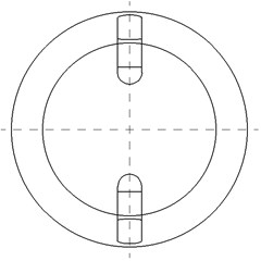
b) Baffle program of scheme 2
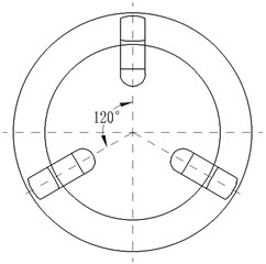
c) Baffle program of scheme 3
3. Mathematical models and numerical simulations
3.1. Mathematical models
For unsteady flow of incompressible fluid, the equation of continuity equation and moment conservation equations can be written as follows:
where is the static pressure, is the density and (1, 2, 3) is fluid velocity. is the molecular viscosity. is Reynolds stress.
Two-equation turbulence models allow the determination of both, a turbulent length and time scale by solving two separate transport equations. The RNG - was adopted in the research. The turbulence kinetic energy, , and its rate of dissipation, , are obtained from the following transport equations:
In these equations, represents the generation of turbulence kinetic energy due to the mean velocity gradients. This term may be defined as . is the generation of turbulence kinetic energy due to buoyancy and is given by . represents the contribution of the fluctuating dilatation in compressible turbulence to the overall dissipation rate, which is defined as , where is the turbulent Mach number, defined as , and is the speed of sound. The quantities and are the inverse effective Prandtl numbers for and , respectively. and are user-defined source terms. , .
3.2. Geometry and grid
Fluid domains of physical model were built by 3D modeling commercial software Creo 3.0. The grids of the geometry model were generated by the manufacturing code ANSYS ICEM. In order to guarantee fluid development enough, the length of inlet extension is 5 times inlet diameter of the centrifugal pump, and the outlet extension length is as 10 times as outlet diameter of the volute. The whole flow passage model with inlet extension, suction chamber, clearance of wear-ring, impeller, volute casing and outlet extension was employed to obtain precise calculation data. The thickness of wear ring clearance in the calculation is 0.2 mm. Hexahedral cells were generated in the inlet, outlet, impeller and wear-ring clearance zones. Unstructured tetrahedral cells were used to define the volute casing because of its complex geometric structure. The grids near tongue zone of volute were refined so as to gain precise unsteady flow structures. Computational model and grids of low specific centrifugal pump are shown in Fig. 2.
Fig. 2Computational model and grids of low specific centrifugal pump
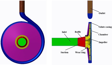
a) Computational model of low specific centrifugal pump
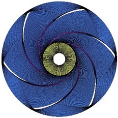
b) The mesh of impeller
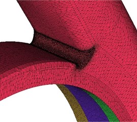
c) The mesh of volute
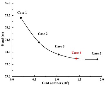
A detailed mesh sensitivity analysis of computational domain was performed so as to eliminate the influence of mesh factor. The same topological structure of computational domain was employed for the research model. Five schemes of grids were gained at the same premise of mesh quantity. The numbers of grids for five cases were 213 000, 642 000, 1 046 000, 1 435 000, 1 973 000, respectively.
The value of head was for the qualitative dimensions of mesh independent check, and the computational head value of five cases were 75.4 m, 74.3 m, 73.9 m, 73.6 m, 73.7 m, respectively. As can be observed in Fig. 3, the head value was gradual decline with the number of girds increasing. Apparent, the head value of case 4 and case 5 were almost the same. It indicates that it will be little impact on numerical results to increase the number of grids from those of case 4. Taking the computer resources in account and keeping the cost under control, the girds numbers of case 4 were chosen to calculate the computational domain.
Fig. 3Mesh sensitivity analysis
3.3. Boundary condition and solution method
The inlet boundary condition of the model pump was defined as velocity-inlet while the outlet boundary condition was set up as pressure-outlet. The Hydraulic diameter of the low specific centrifugal is 50 mm and the value of turbulence intensity was calculated directly [18]. Sliding mesh technology was employed to deal with the information transfer between the rotating impeller and the stationary volute. The walls of the model pump were defined as no-slip condition, and the standard wall function was used to solve the low Reynolds number flow in the near wall region. Commercial software Fluent based on the finite volume method was employed to simulate unsteady flow field in the low specific centrifugal. SIMPLEC algorithm was adopted to calculate pressure-velocity coupling.
In order to obtain detailed resolution of unsteady flow results of the low specific centrifugal pump, time step of the unsteady calculation should satisfy the Courant number criterion [19]:
where is the absolute value of the estimated average velocity. is the smallest size of the grid. Considering the scale of grid and impeller speed of the model pump, time step was set as 5.65×10⁻⁵, which indicate that each impeller revolution will be calculated in a time sequence of 360 times steps corresponding to 1° of the impeller rotation speed. The numerical residual convergence criterion was set as 10-5 so as to ensure the result to be converged. To obtain a rapid convergence process, steady simulation was first carried out in advance, which was set as the initial condition for transient calculation.
4. Results and discussions
4.1. Performance characteristics analysis
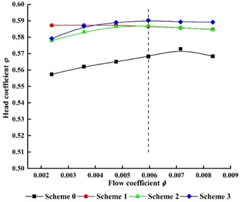
Comparison of head value for four schemes are shown in Fig. 4. Flow at the dashed is operation flow rate ( 0.00596). As can be seen in Fig. 4, with the increase of flow rate, the head value of four schemes increases first and then decreases. Namely, there is a hump phenomenon in the low specific speed centrifugal pump.
It is easily found the head value of no baffle in the suction (scheme 0) is lower than that with baffles in the suction (scheme 1, scheme 2, scheme 3) at each condition point. Hump point in scheme 0 is at 0.00596 (1.2 times ). The hump point in scheme 1, scheme 2, scheme 3 is at 0.8, 1.0, 1.0, respectively. It indicates that the baffle in the suction can affect the inlet flow pattern of the impeller and further impact the energy distribution in the impeller.
Fig. 4External characteristics curves for four schemes
In order to measure the hump degree in each scheme, the dimensionless formula is introduced as follows:
where is the head coefficient at hump point for scheme . is the head coefficient at 0.002383 for four schemes. 0, 1, 2.3; 0, 1, 2, 3. The comparison of and for four schemes are is list in Table 2.
Table 2The comparison of ε for four schemes
Scheme | ||||
0 | 0.57287 | 0.55738 | 2.704 % | 159 |
1 | 0.58729 | 0.58719 | 0.017 % | 1 |
2 | 0.58691 | 0.57791 | 1.533 % | 90 |
3 | 0.59022 | 0.57916 | 1.873 % | 110 |
As can be observed in Table 2, the value of scheme 1 is the smallest and scheme 0 one is the largest in the four schemes (159 times scheme 1). The scheme 2 and scheme 3 are 90 times and 110 times scheme 1, respectively. It shows that the number of baffle affect centrifugal pump hump location and intensity, and the best number of baffles in the suction is one.
4.2. Analysis of time domain on monitoring points
In order to explore the pressure pulsation characteristics of the low specific speed centrifugal pump under various schemes in details, thirty-six monitoring points were set up evenly in the volute calculation domains. As shown in Fig. 5, thirty-six monitoring points were all placed in the symmetry plane of the volute, and they were arranged as counter clockwise, which was in the same direction with the impeller rotating. The diameter of base circle the monitoring points on is 230 mm. Angle of monitoring point P1 was defined as 0°.
The static pressure value of numerical simulation on each monitoring point is given at different times. In order to accurately compare the diffidence of pressure on each monitoring point, the pressure coefficient is introduced:
where is the static pressure on the monitoring point. is the average static pressure for the impeller rotating a circle and u is the circumferential velocity of the impeller.
Fig. 5Distribution of pressure pulsation monitoring points
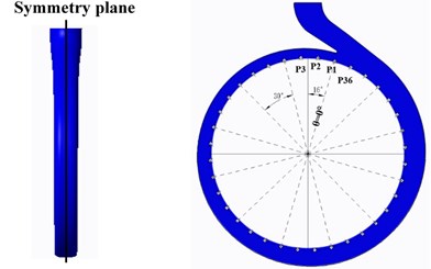
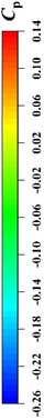
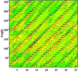
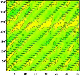
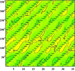
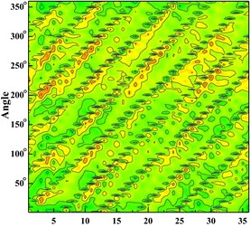
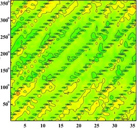
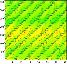
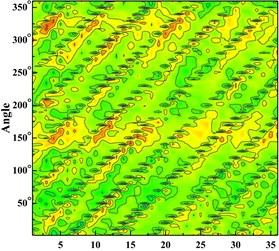
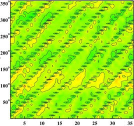
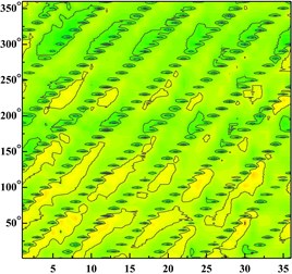
Fig. 6 shows the distribution of the pressure pulsation time domain of thirty-six monitoring points around the impeller at one impeller rotation period. Abscissa represents different monitoring points, and ordinate is angle around volute inlet.
From the Fig. 6 It can be seen that six wave troughs are observed clearly at each monitoring point as the impeller rotates in a circle, which corresponds to the six blades. The appearance of the former trough is earlier than that of the latter one at one impeller channel period. Each time the impeller is turned 10 degrees, there are six obvious troughs around the impeller. It shows that the rotor-stator interaction between the impeller and the volute is the main cause of the pressure pulsation.
With the increase of the flow rate, the pressure fluctuation of each scheme tends to be gradual. The pressure fluctuation in time domain is severe at 0.002383 in four schemes. It is because that the flow rate is much small and there are lots of secondary flow phenomenon in impeller runner.
4.3. Frequency domain analysis on monitoring point
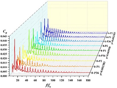
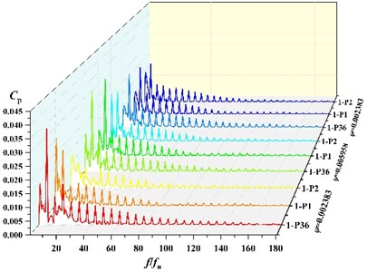
Due to space limitations and taking into account the causes of static and dynamic interference, frequency analysis of three points P36, P1, P2 under different flow condition, which are near the volute tongue, is performed in this section. The frequency distribution of the pressure pulsations coefficients at 3 monitoring points near the tongue is shown in Fig. 7. It can be found that with the rotation of the impeller, peak value of pressure fluctuation at blade passing frequency (BPF) is gradually decrease, which means amplitude on P36 > P1 > P2 at BPF under all schemes. At low flow (0.002383), the main frequency of pressure fluctuation at P36 and P1 under scheme 0, scheme 2 and scheme 3 is 295 Hz, which is corresponding to BPF. The main frequency of P2 under scheme 0, scheme 2 and scheme 3 is 49.17 Hz. At scheme 1, the fluctuation main frequency is 49.17 Hz at P1 and P2, and the main frequency at P36 is 295 Hz, which are shaft frequency and BPF, respectively. It indicates that fluctuation frequency distribution around impeller is affected by the suction baffles distribution. Under other flow rates, the main frequency of pressure fluctuation at three points is 295 Hz.
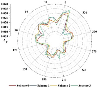
Fig. 8 shows the comparison of fluctuation amplitude at BPF for each point. It can be found that with the change of angle, the peak of pressure fluctuation at BPF in the volute varies periodically. The maximum value of amplitude is all at 360° of the volute (at P36 location). The minimum value of amplitude is all near 150°. Seven peaks and troughs of amplitude are captured. It indicates that amplitude of frequency at BPF is in periodic fluctuations.
Fig. 6Time domain diagram of monitoring point: a) time domain diagram of scheme 0 at ϕ= 0.002383; b) time domain diagram of scheme 0 at ϕ= 0.005958; c) time domain diagram of scheme 0 at ϕ= 0.008342; d) time domain diagram of scheme 1 at ϕ= 0.002383; e) time domain diagram of scheme 1 at ϕ= 0.005958; f) time domain diagram of scheme 1 at ϕ= 0.008342; g) time domain diagram of scheme 2 at ϕ= 0.002383; h) time domain diagram of scheme 2 at ϕ= 0.005958, i) time domain diagram of scheme 2 at ϕ= 0.008342; j) time domain diagram of scheme 3 at ϕ= 0.002383; k) time domain diagram of scheme 3 at ϕ= 0.005958; l) time domain diagram of scheme 3 at ϕ= 0.008342
a)
b)
c)
d)
e)
f)
g)
h)
i)
In order to evaluate the influence of baffle on the pressure fluctuation level of the low specific speed pump, formula of decrease rate for pressure fluctuation is introduced as follows:
where is the average value of pressure fluctuation coefficient at BPF, 0, 1, 2, 3.
Fig. 7Frequency distribution of three points at different scheme
a) Frequency distribution of three points at scheme 0
b) Frequency distribution of three points at scheme 1
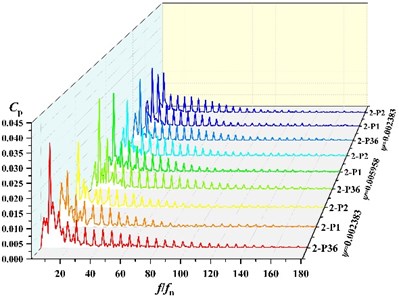
c) Frequency distribution of three points at scheme 2
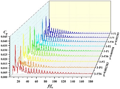
d) Frequency distribution of three points at scheme 3
Fig. 8Comparison of fluctuation amplitude at BPF for each point
As can be observed in Table 3, the pressure fluctuation levels were decreased by –2.72 %, –2.13 %, and –2.21 % respectively when the number of baffle in the suction is one, two, three. And of scheme 1 is maximum. It indicates that Adding a baffle to the suction chamber is beneficial to reduce the amplitude of pressure pulsation at BPF in the volute. The best number of baffles in the suction is one.
Table 3Mean pressure fluctuation amplitude at BPF
Scheme | Frequency (Hz) | ||
0 | 295 | 0.01779 | 0 |
1 | 295 | 0.01732 | –2.72 % |
2 | 295 | 0.01742 | –2.13 % |
3 | 295 | 0.01741 | –2.21 % |
5. Test verification
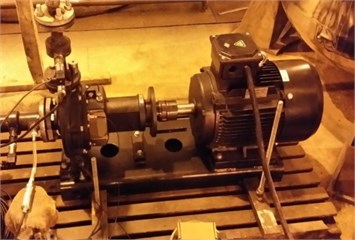
The suction of prototype was designed based on the scheme 1 simulation results, and the performance test was performed. Fig. 9 shows the model pump geometry profile and the physical drawing of the prototype is shown in Fig. 10.
Fig. 9Model pump geometry profile: 1 – suspension, 2 – rear pump cover, 3 – impeller, 4 – inlet flange, 5 – baffle, 6 – pump shaft, 7 – mechanical seal, 8 – bracket
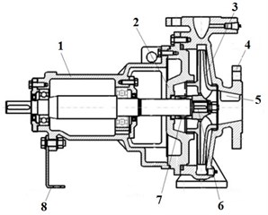
Fig. 10Physical drawing of model pump
Performance experiments of the low centrifugal pump were performed in a closed-loop test platform schematized in Fig. 11(a). The model pump was driven by a variable speed electric AC motor controlled by a frequency converter. The water was pumped from and returned to reservoir. The shaft torque and rotational speed were monitored by a torque and speed sensor with errors under ±0.10 %. Static pressure values were measured at the inlet and outlet of the pump by a differential pressure transfer, and the uncertainty was within ±0.10 %. The flow rate was measured by a magnetic flow meter with the uncertainty less than ±0.14 %. The measurement accuracy of pump efficiency was quantified as ±0.30 %. Scheme and physical map of the test rig are shown in Fig. 11.
Fig. 12. shows the Contrast of head and efficiency between simulation and experiment. The numerical results are compared with experimental results of the super low specific speed centrifugal pump designed by increasing flow method so as to validate the reliability of CFD. Q-H and Q- curve of the model pump is presented in Fig. 12. A good agreement of the head between numerical results and experimental results are observed. The head value of simulation and experiment at operational flow rate (labeled at dotted line) are 73.74 m, 75.57 m, respectively. The relative head error between calculation and experiment values is less than 5 % under all flow rate. The maximum absolute error value of efficiency is no more than 2.3 %. It is worth mentioning that in order to ensure the repeatability of the test results, the experiment was performed 3 times, and the experimental data were averaged over 3 times. No hump was captured from the H-Q curve of the experiment.
Fig. 11Scheme and physical map of the test rig
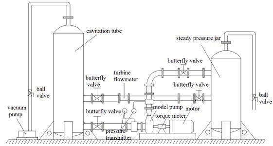
a) Scheme of the test rig
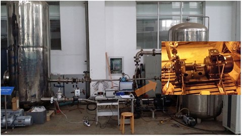
b) Physical map of the test rig
Fig. 12Contrast of head and efficiency between simulation and experiment
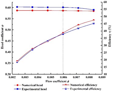
The efficiency curves between numerical results and experimental results are monotone increasing with flow rate increasing. This is because that the model pump was designed by enlarging flow method and the maximum flow point presented in Fig. 12 don’t reach the nominal flow rate (30 m3/h) Efficiency value of the simulation and test at operational flow rate are 38.66 %, 37.88 %, respectively. It indicts that the calculation is feasible for the model pump and can be used to perform detail analysis.
6. Conclusions
In this paper, a low specific speed centrifugal pump was designed based on the enlarged flow method. Four schemes were designed to research the effect of baffles on performance and unsteady characteristics of pressure fluctuations of centrifugal pump, and some conclusions are taken as follows:
1) The head value of no baffle in the suction is lower than that with baffles in the suction at each condition point. Hamp point in scheme 0 is at 0.00596 (1.2 times ). The hump point in scheme 1, scheme 2, scheme 3 is at 0.8, 1.0, 1.0, respectively. The value of scheme 1 is the smallest and the scheme 0 one is the largest in the four schemes (159 times scheme 1). The scheme 2 and scheme 3 are 90 times and 110 times scheme 1, respectively. The best number of baffles in the suction is one.
2) Six wave troughs are observed clearly at each monitoring point as the impeller rotates in a circle, which corresponds to the 6 blades. The appearance of the former trough is earlier than that of the latter one at an impeller channel period. Each time the impeller is turned 10 degrees, there are six obvious troughs around the impeller. It shows that the rotor-stator interaction between the impeller and the volute is the main cause of the pressure pulsation.
3) With the rotation of the impeller, peak value of pressure fluctuations at blade passing frequency (BPF) is gradually decrease, which means amplitude on P36 > P1 > P2 at BPF under all schemes. At low flow (0.002383), the main frequency of pressure fluctuation at P36 and P1 under scheme 0, scheme 2 and scheme 3 is 295 Hz, which is corresponding to BPF. the main frequency of P2 under scheme 0, scheme 2 and scheme 3 is 49.17 Hz. At scheme 1, the fluctuation main frequency is 49.17 Hz at P1 and P2, and the main frequency at P36 is 295 Hz, which are shaft frequency and BPF, respectively.
4) The pressure fluctuation levels were decreased by –2.72 %, –2.13 %, and 2.21 % respectively when the number of baffle in the suction is one, two, three, respectively. And of scheme 1 is maximum. It indicates that Adding a baffle to the suction chamber is beneficial to reduce the amplitude of pressure pulsation at BPF in the volute. The best number of baffles in the suction is one.
References
-
Yuan S. Q. Theory and Design of Low Specific Speed Centrifugal Pump. China Machine Press, Beijing, 1997.
-
Pei J., Wang W. J., Yuan S. Q., et al. Optimization on the impeller of a low-specific-speed centrifugal pump for hydraulic performance improvement. Chinese Journal of Mechanical Engineering, Vol. 29, Issue 5, 2016, p. 992-1002.
-
Liu H. L., Luo K. K., Wu X. F., et al. Effect of inlet splitter on pressure fluctuations in a double-suction centrifugal pump. Journal of Vibroengineering, Vol. 19, Issue 1, 2017, p. 549-562.
-
Gao B., Zhang N., Li Z., et al. Influence of the blade trailing edge profile on the performance and unsteady pressure pulsation in a low specific speed centrifugal pump. Journal of Fluids Engineering, Vol. 138, Issue 5, 2015, p. 51106.
-
Li W., Shi W. D., Jiang T., et al. Analysis on effects of the blade wrap angle and outlet angle on the performance of the low-specific speed centrifugal pump. Advanced Materials Research, Vol. 354, 2012, p. 615-620.
-
Zhang Y. L., Zhu Z. C., Li W. G. Experiments on transient performance of a low specific speed centrifugal pump with open impeller. Proceedings of the Institution of Mechanical Engineers, Part A: Journal of Power and Energy, Vol. 230, Issue 7, 2016, p. 648-659.
-
Zhang J. F., Wang Y. F., Yuan S. Q. Experimental research on internal flow in impeller of a low specific speed centrifugal pump by PIV. Materials Science and Engineering, Vol. 129, Issue 1, 2016, p. 12013.
-
Zhang N., Yang M. G., Gao B., et al. Investigation of rotor-stator interaction and flow unsteadiness in a low specific speed centrifugal pump. Strojniški Vestnik-Journal of Mechanical Engineering, Vol. 62, Issue 1, 2016, p. 21-31.
-
Wang W. J., Wang Y. Analysis of inner flow in low specific speed centrifugal pump based on LES. Journal of Mechanical Science and Technology, Vol. 27, Issue 6, 2013, p. 1619-1626.
-
Gao B., Guo P., Zhang N., et al. Unsteady pressure pulsation measurements and analysis of a low specific speed centrifugal pump. Journal of Fluids Engineering, Vol. 139, Issue 7, 2017, p. 71101.
-
Cui B. L., Chen D. S., Xu W. J., et al. Unsteady flow characteristic of low-specific-speed centrifugal pump under different flow-rate conditions. Journal of Thermal Science, Vol. 24, Issue 1, 2015, p. 17-23.
-
Zhu B., Chen H. X., Wei Q., et al. The analysis of unsteady characteristics in the low specific speed centrifugal pump with drainage gaps. Earth and Environmental Science, Vol. 15, Issue 3, 2012, p. 32049.
-
Fu Q., Yuan S. Q., Zhu R. S. Pressure fluctuation of the low specific speed centrifugal pump. Applied Mechanics and Materials, Vol. 152, 2012, p. 935-939.
-
Alemi H., Nourbakhsh S. A., Raisee M., et al. Effects of volute curvature on performance of a low specific-speed centrifugal pump at design and off-design conditions. Journal of Turbomachinery, Vol. 137, Issue 4, 2015, p. 41009.
-
Alemi H., Nourbakhsh S. A., Raisee M., et al. Effect of the volute tongue profile on the performance of a low specific speed centrifugal pump. Proceedings of the Institution of Mechanical Engineers, Part A: Journal of Power and Energy, Vol. 229, Issue 2, 2015, p. 210-220.
-
Zhang X., Wang Y., Fu J. H., et al. Effect of the section area of volute in low specific speed centrifugal pumps on hydraulic performance. Fluids Engineering Division Summer Meeting, 2009, p. 41-50.
-
Gülich J. F. Centrifugal Pumps. Springer, Berlin Heidelberg, 2010.
-
Wang F. J. Computational Fluid Dynamics Analysis – CFD Software Principle and Application. Tsinghua University Press, Beijing, 2004.
-
Shi F., Tsukamoto H. Numerical study of pressure fluctuations caused by impeller-diffuser interaction in a diffuser pump stage. Journal of Fluids Engineering, Vol. 123, Issue 3, 2001, p. 466-474.
Cited by
About this article

The authors would like to thank the support by the National Natural Science Foundation of China (51239005, 51779106), Jiangsu Industry University Research Cooperation Innovation Fund – Forward Joint Research Project (BY2015064-10), Priority Academic Program Development of Jiangsu Higher Education Institutions (PAPD), Open subject of Key Laboratory of Fluid and Power Machinery, Ministry of Education, Xihua University. (szjj2016-068), Jiangsu Top Six Talent Summit Project (GDZB-017).
Kaikai Luo performed the data analyses and wrote the manuscript. Yong Wang conceived and designed the experiments. Houlin Liu contributed to the conception of the study. Jie Chen helped perform the analysis with constructive discussions. Yu Li helped carry out experiments. Jun Yan contributed significantly to analysis and manuscript preparation.
