Analysis of dynamic response law and time-frequency characteristics of high cut slope under the action of earthquake

Jin, Honghua; Wang, Linfeng; Ren, Qingyang; Zhang, Xingxing

doi:10.21595/jve.2021.21764

Journal of Vibroengineering

Browse Journal

Submit article

Published: 19 February 2021

Check for updates

Analysis of dynamic response law and time-frequency characteristics of high cut slope under the action of earthquake

Honghua Jin¹

Linfeng Wang²

Qingyang Ren³

Xingxing Zhang⁴

^{1, 3}State Key Laboratory of Mountain Bridge and Tunnel Engineering, Chongqing Jiaotong University, Chongqing, 400074, China

²Key Laboratory of Geological Hazards Mitigation for Mountainous Highway and Waterway, Chongqing Municipal Education Commission, Chongqing Jiaotong University, Chongqing, 400074, China

⁴School of Civil Engineering, Chongqing University of Arts and Science, Chongqing, 402160, China

Corresponding Author:

Linfeng Wang

Cite the article Download PDF

Downloads 1046

Abstract

This study aimed to reveal the dynamic response law and time-frequency characteristics of the slope under the action of earthquake. Based on an actual project in earthquake area, the stability of the slope under natural and seismic conditions was calculated and the meso parameters of rock and soil were obtained by indoor rock and soil specimen parameter test firstly. Meanwhile, a three-dimensional particle flow model of the high-cut slope was established by the three-dimensional particle flow software PFC3D. Then, the law of dynamic response of the slope acceleration was obtained by inputting the horizontal wave of 2008 Wenchuan earthquake. Furthermore, MATLAB programming was used to analyze the time-history signal of acceleration of the slope, and finally the time-frequency characteristics of the high cut slope under the action of earthquake were studied. The results show that the dynamic response characteristics of soil particles in horizontal and vertical directions show surface-tending effect and elevation amplification effect respectively under the action of earthquake. The analysis of time-frequency characteristics showed that the Fourier dominant frequency of soil particles is distributed between 0-5 Hz under the action of earthquake, the low frequency band (0-15.625 Hz) accounts for as high as 88.07 %, and the high frequency band (125-250 Hz) accounts for as low as 0.34 %.

Analysis of dynamic response law and time-frequency characteristics of high cut slope under the action of earthquake

1. Introduction

In recent years, with the rapid development of infrastructure construction in China, especially the large-scale construction of large-scale transportation projects in the mountainous areas of Sichuan and Chongqing in southwest China, has resulted in increasing problems of the stability of rock and soil slopes. The southwestern mountainous area is surrounded by mountains, and high mountains, deep valleys, steep topography, special and complex geological structures and topographic conditions. Highway engineering must be built on the mountain. Due to the constraints of local economic development, traffic demand, road grade requirements, financial investment and other factors, most of the engineering slopes often form high cut slopes of several kilometers at the foot of the mountain, which lacks effective support measures. Moreover, Sichuan-Chongqing area in Southwest China is located in the Helan Mountain-Liupan Mountain-Longmen Mountain-Hengfault Mountain fault zone where earthquake disasters are frequent. A large number of slope engineering without support measures are unstable under the action of earthquake, which often causes huge economic and property losses. The existing studies mostly focus on the stability analysis of natural slopes in the earthquake area, and mainly focus on the stability calculation and failure mechanism. For the study of seismic vibration hazards, from the perspective of structural dynamics, the influence of vibration frequency and vibration velocity on the structure is equally important. At present, there are few researches based on the dynamic response law of slopes, and the research on the vibration frequency of seismic slopes needs to be solved urgently. Especially, taking the artificial soil high cut slope in earthquake area as the research object, the research on the dynamic response law and time-frequency characteristics of the high cut slope under the action of earthquake has gradually become one of the research hotspots and technical problems in this field.

In the aspect of dynamic response law of slope, Lin et al. [1] used large-scale shaking table model test to simulate the dynamic response of homogeneous sand slope under earthquake action by inputting sine waves with different frequencies and accelerations. Debabrata Giri et al. [2] conducted a shaking table test on a small embankment slope to study its dynamic characteristics. Based on the characteristics of concentrated deformation and failure of excavation damaged slope in Wenchuan earthquake, A et al. [3] took granite as the finite element model of excavation damaged slope, and takes 45° natural slope as an example to study the excavation failure effect and seismic dynamic response of different excavation angles under certain conditions. Zhang [4] took the soil slope as the research object and comprehensively considered the characteristics of the soil slope and ground motion to analyze and evaluate the seismic dynamic response law and stability of the soil slope. Tang [5] took the plateau highway in Ganzi section of China National Highway G317 as the engineering background, and revealed the displacement and deformation of the slope and the dynamic response of acceleration inside the slope under the action of different seismic waves by designing the indoor vibration table model of the soil layered slope. Based on the finite element numerical simulation method, Zhang et al. [6] established a two-dimensional homogeneous finite element model of slope, simulated and analyzed the acceleration and displacement response of slope models under different seismic actions, and revealed the law of the influence of peak acceleration, frequency spectrum and duration of ground motion on the seismic response of soil slope. Deng [7] combined centrifugal vibration test and three-dimensional discrete element numerical simulation method to analyze and explore the dynamic response characteristics and instability mechanism of the steeply inclined soft and hard bedding slope in the Wenchuan earthquake area. Zhao et al. [8] took the 7th block of Landslide Group 0# of Yushu Airport Road, China as the research object, and took the large finite element analysis software FLAC3D as the research tool to study the dynamic response law of landslide under different acceleration peak effects of Seismic wave, Yushu horizontal wave and Yushu vertical wave. Taking the typical stepped loess slope as the research object, Yan et al. [9] established the numerical simulation model data program with flac3 to study the dynamic response of different shapes of loess slope. Chen et al. [10] conducted a large-scale shaking table model test on a pure loess slope in Lanzhou New District, China as a prototype to study the dynamic response law and failure mechanism of pure loess slope under seismic load. In the aspect of time-frequency characteristic analysis of slope, Yang et al. [11] adopted a new discrete element method based on continuity to simulate the whole process of slope from initial deformation to sliding in the process of surface vibration, and used the Hilbert-Huang transformation to analyze the causes of induced landslide in the combined time-frequency domain. Fan et al. [12, 13] considered the time-frequency characteristics of seismic waves and based on the Hilbert-Huang transformation and the large shaking table test, a dynamic method based on energy to analyze the seismic stability of rock slope was proposed. Song et al. [14] used the finite element method to study the dynamic response of rock slopes with discontinuous structural planes, and proposed a time-frequency joint analysis method combining time-frequency and time-frequency domain analysis, which clarified the seismic response of rock slopes.

The above researches on dynamic response of slope under the action of earthquake are mostly based on single inclined homogeneous soil slopes, and most of the researches on slope frequency band and energy based on time-frequency theory are focused on rock slope. Moreover, the two-dimensional finite element method is often used in the process of numerical simulation. Due to the complexity and long operation time of 3D discrete element method, the research on dynamic response law and frequency band energy distribution of slope in 3D state is still in its infancy stage. Therefore, for the common bedrock stepped soil high slope in seismic area, its applicability is relatively low, and the laws of seismic dynamic response and frequency band energy distribution are poorly understood. Based on this, this paper took the two-stage bedrock-type high cut slope with silty clay overburden as the research object, and obtained the meso parameters of rock and soil through indoor triaxial test and the PFC numerical triaxial servo test. A three-dimensional particle flow numerical model of this type of high cut slope was established based on the PFC3D three-dimensional discrete element software. By introducing 2008 Wenchuan earthquake wave, the acceleration dynamic response law of this kind of slope under the action of earthquake was obtained. The frequency spectrum analysis of the vibration acceleration time history signal of the slope was carried out by using MATLAB programming, and the dynamic response and frequency band energy distribution of this kind of slope under the action of earthquake was revealed.

In view of the sudden and catastrophic characteristics of high cut slope failure under the action of earthquake, a simplified analysis method of high cut slope stability under the action of earthquake was established, and the dynamic response law and time frequency characteristics were revealed in this paper, the research results provides a theoretical basis for the stability evaluation, prevention and prediction of this kind of high cut slope in earthquake area under the action of earthquake, and have important scientific guiding significance and practical value for the safety of people’s lives and property and the safe operation of major infrastructure in the earthquake area.

2. Selection of research sites

In this paper, the right side of k41 + 538 ~ k41 + 615 section A1 of Mabian Zhaojue section of Lexi Expressway in Sichuan Province of China was taken as the research object. Its seismic intensity is VIII degree, the peak acceleration value of ground motion is 0.2 g. The study area is located near Luoshan river in Mabian County, Leshan City, Sichuan Province, China. The overall landform type belongs to tectonic erosion and denudation hilly landform. The slope body is mainly composed of quaternary Holocene residual slope silty clay (Q₄^dl+el), with the soil thickness of 6.0-13.0 m, soft plastic-plastic. The lower impermeable bedrock is the Jurassic mudstone of Suining Formation (J_2S), most of which are strongly weathered to moderately weathered. Preliminary investigation shows that the groundwater level is far lower than the bottom of the bedrock. This construction site is planned to adopt a two-stage platform excavation method, with single-stage slope height of 8 m and slope ratio of 1:1.00, a platform width of 2 m at the junction of the two-stage slopes, a slope angle of 45°, and an impervious bedrock surface inclination angle of 30°. The mechanical parameters of soil are shown in Table 1.

Fig. 1The real scene and the geological profile of the high cut slope roadbed at the research site

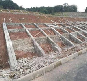
a) The real scene

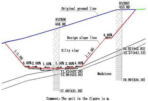
b) The geological profile

Table 1Physical and mechanical parameters of silty clay and mudstone

Category	Parameter
Category	$γ$ (kN/m³)	$c$ (kPa)	$φ$ (°)	Natural water content (%)	Saturation permeability coefficient $k_{s}$ (cm/s)	Saturated water content $θ_{s}$	Residual water content $θ_{r}$
Silty clay	18.5	33.6	24.8	10.27	5.0×10^-5	0.46	0.08
Mudstone	25.2	716.42	27.51	–	–	–	–

3. High cut slope stability calculation

3.1. Natural conditions

3.1.1. Analysis of soil stress state of slope

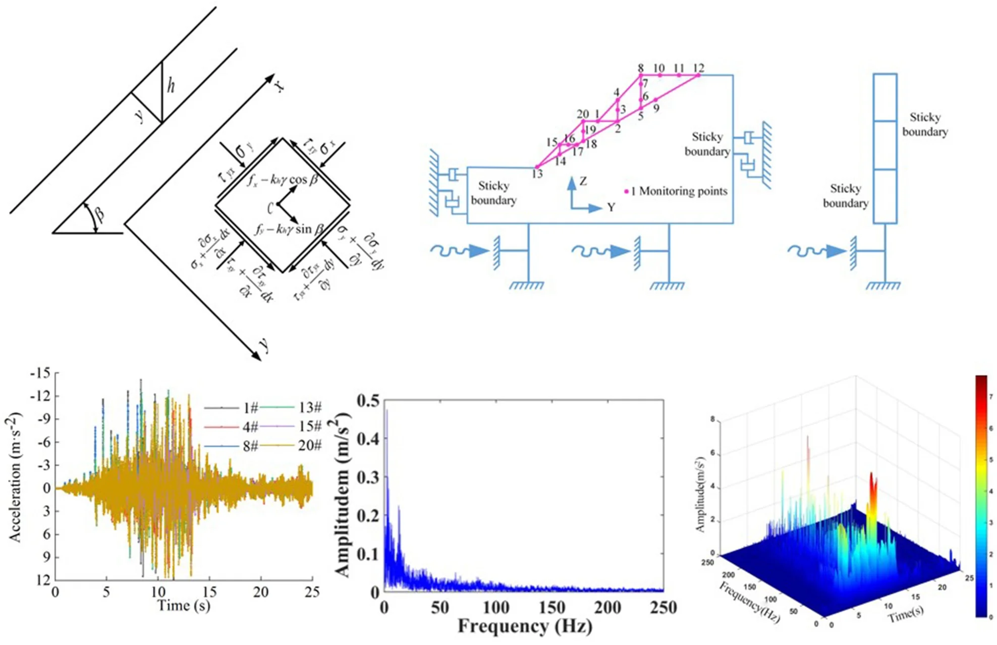
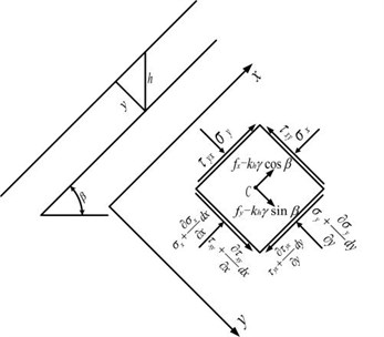
Generally speaking, the two-dimensional problem in soil are often regarded as plane strain problem due to the impossibility of cutting the soil into thin slices [15]. In this paper, the stress analysis of any micro element in an infinite homogeneous soil slope can be simplified as a two-dimensional plane strain problem, and its stress state is shown in Fig. 2.

Fig. 2Stress state of slope soil under natural conditions

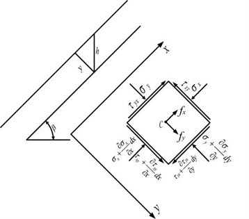
Based on the theory of elasticity, geometry and statics, a rectangular coordinate system was established with the direction of the slope surface as the $X$ -axis and the direction perpendicular to the slope surface as the $Y$ -axis. The equilibrium differential equation is as follows:

1

\frac{\partial σ_{x}}{\partial x} + \frac{\partial τ_{y x}}{\partial y} - γ s i n β = 0,

2

\frac{\partial σ_{y}}{\partial y} + \frac{\partial τ_{x y}}{\partial x} - γ c o s β = 0,

where, $σ_{x}$ and $σ_{y}$ are the normal stress components along the tangent and normal directions of the soil micro-element, respectively. $τ_{y x}$ and $τ_{x y}$ are the shear stress components along the tangent and normal directions, respectively. $γ$ is the soil weight, $β$ is the slope angle.

Relative to the distance from the slope to the potential sliding surface, it can be assumed that the slope is homogeneous and infinite long along the slope direction, that is, the slope tends to be infinitely long along the $X$ -axis direction, then the magnitude and distribution of stress on any cross section of the slope are the same. Therefore, $σ_{x}$ is only a function of y which is independent of $x$ , that is, $\partial σ_{x} / \partial_{x} =$ 0, and considering the boundary conditions $τ_{y x} |_{y = 0} = 0$ [16], then:

3

τ_{y x} = γ y s i n β .

Because $y = h c o s β$ , and then substituting Eq. (3) into Eq. (2), we can get that:

4

σ_{y} = γ h c o s^{2} β,

where, $h$ is the depth of soil micro element.

Based on the theory of soil mechanics, the following conclusions can be obtained:

5

σ_{x} = λ σ_{y} = λ γ h c o s^{2} β,

where, $λ$ is a constant, $λ = v / (1 - v)$ , and $v$ is Poisson’s ratio.

According to soil mechanics, the normal stress $σ_{1}$ and $σ_{3}$ are respectively [17]:

6

σ_{1}, σ_{3} = \frac{σ_{x} + σ_{y}}{2} \pm \sqrt{{(\frac{σ_{x} - σ_{y}}{2})}^{2} + τ_{x y}^{2}} .

By integrating Eq. (4) and Eq. (5) into Eq. (6), the normal stress $σ_{1}$ and $σ_{3}$ can be converted into:

7

σ_{1}, σ_{3} = \frac{γ h}{2} ((λ + 1) c o s^{2} β \pm \sqrt{(λ - 1)^{2} c o s^{4} β + s i n^{2} 2 β}) .

Based on soil mechanics, the cohesive strength of soil ( $c$ ) is as follows:

8

c = \frac{(σ_{1} - σ_{3}) - (σ_{1} + σ_{3}) s i n φ}{2 c o s φ},

where, $φ$ is the friction angle of the soil.

In Eq. (7), $λ$ and $β$ are both constants, it can be considered that normal stress $σ_{1}$ and $σ_{3}$ are linear functions of $γ h$ , that is:

9

σ_{1} = k_{1} γ y, σ_{3} = k_{2} γ y,

where:

k_{1} = \frac{1}{2} ((λ + 1) c o s^{2} β + \sqrt{(λ - 1)^{2} c o s^{4} β + s i n^{2} 2 β}),

k 2 = \frac{1}{2} ((λ + 1) c o s^{2} β - \sqrt{(λ - 1)^{2} c o s^{4} β + s i n^{2} 2 β}) .

Then $c$ can be simplified as:

10

c = γ h (\frac{k 1 - k 2 - (k_{1} + k_{2}) s i n φ}{2 c o s φ}) .

3.1.2. Calculation of slope stability coefficient

In this paper, Geo-studio numerical simulation software and Lizheng geotechnical calculation software were used to automatically search for the most dangerous sliding surface to calculate the initial stability coefficient of the slope. The calculation results are shown in Table 2. It can be seen that the numerical simulation result of Geo-Studio software is 2.451, and the Lizheng geotechnical calculation result takes the average of the three of 2.326, which is 95 % of the former. Considering the error of the numerical simulation process, there is no significant difference between them, and the high cut slope is stable in natural state.

Table 2Calculation table of initial stability coefficient of high cut slope

Calculation software	Calculation method	Stability coefficient	Calculation software	Calculation method	Stability coefficient software
Geo-studio	Slope / W	2.451	Lizheng Geotechnical Calculation	Swedish Article Law	2.252
				Simplified Bishop method	2.268
				Janbu method	2.458

3.2. Earthquake conditions

3.2.1. Analysis of soil stress state of slope

For the stability calculation of high cut slope under the action of earthquake, the seismic pseudo-static method combined with the limit equilibrium method is commonly used in the existing literature. This method is simple and clear, but the calculation process is complicated and the amount of calculation is long, which is not convenient for engineers and technicians to use. In this paper, in order to simplify the impact of seismic action on the stability of high cut slope, based on the analysis of the soil stress state under the action of earthquake, the seismic force was firstly simplified as the equivalent relationship of the difference between the ultimate cohesive strength ( $c'$ ) of slope body under the action of earthquake and the initial effective cohesive strength ( $c''$ ). Then, the calculation methods of the ultimate cohesive strength ( $c'$ ) and equivalent cohesive strength ( $c''$ ) of the slope body under the action of earthquake were established, and the simplified analysis method of the influence of earthquake action on the stability of the high cut slope was proposed, which was applied to the actual engineering case in this paper.

Many studies have shown that the vertical seismic force has little influence on the slope stability. Therefore, the pseudo-static method was used to calculate the horizontal seismic force $F_{x}$ without considering the vertical seismic force [18]:

11

F x = k h W,

where, $F_{x}$ is horizontal seismic force, $k_{h}$ is the coefficient of horizontal seismic action, $W$ is the weight of soil.

Referring to the analysis process of slope soil stress state under natural state in the previous section, any micro-element in an infinite homogeneous soil slope was selected for stress analysis, and the stress state of micro element is shown in Fig. 3. Accordingly, the equilibrium differential equation of soil micro-element under the action of earthquake can be rewritten as follows:

12

\frac{\partial σ_{x}^{'}}{\partial x} + \frac{\partial τ_{y x}^{'}}{\partial y} - γ (s i n β + k h c o s β) = 0,

13

\frac{\partial σ_{y}^{'}}{\partial y} + \frac{\partial τ_{x y}^{'}}{\partial x} - γ (c o s β + k h s i n β) = 0,

where, $σ_{x}^{'}$ and $σ_{y}^{'}$ are the normal stress components along the tangent and normal directions of the soil micro-element under the action of earthquake, respectively. $τ_{y x}^{'}$ and $τ_{x y}^{'}$ are the shear stress components along the tangent and normal directions under the action of earthquake, respectively.

Then, Eq. (3) can be rewritten as:

14

τ'_{y x} = γ y (s i n β + k h c o s β) .

Substituting Eq. (14) into Eq. (13):

15

σ_{y}^{'} = γ h （c o s^{2} β + k h s i n β c o s β）,

16

σ_{x}^{'} = λ σ_{y}^{'} = λ γ h （c o s^{2} β + k h s i n β c o s β） .

Substituting Eq. (15) and Eq. (16) into Eq. (6), then the normal stress $σ_{1}^{'}$ and $σ_{3}^{'}$ are:

17

σ_{1}^{'}, σ_{3}^{'} = \frac{γ h}{2} ((λ + 1) (c o s^{2} β + k h s i n β c o s β)

\pm \sqrt{(λ - 1)^{2} (c o s^{2} β + k h s i n β c o s β)^{2} + 4 (s i n β c o s β + k h c o s^{2} β)^{2}}) .

In Eq. (17), $λ$ , $β$ and $k h$ are both constant, therefore, it can be considered that normal stress $σ_{1}^{'}$ and $σ_{3}^{'}$ are linear functions of $γ h$ , that is:

18

σ_{1}^{'} = k 3 γ y, σ_{3}^{'} = k 4 γ y,

where:

k_{3} = \frac{1}{2} ((λ + 1) (c o s^{2} β + k h s i n β c o s β)

+ \sqrt{(λ - 1)^{2} (c o s^{2} β + k h s i n β c o s β)^{2} + 4 (s i n β c o s β + k h c o s^{2} β)^{2}}),

k_{4} = \frac{1}{2} ((λ + 1) (c o s^{2} β + k h s i n β c o s β)

- \sqrt{(λ - 1)^{2} (c o s^{2} β + k h s i n β c o s β)^{2} + 4 (s i n β c o s β + k h c o s^{2} β)^{2}}),

Fig. 3Stress state of slope soil under the action of earthquake

Then the cohesive strength required ( $c'$ ) when the slope reaches the limit equilibrium state under the action of earthquake is as follows:

19

c^{'} = γ h (\frac{k 3 - k 4 - (k 3 + k 4) s i n φ}{2 c o s φ}) .

The variation of normal stress $σ_{1}^{'}$ and $σ_{3}^{'}$ at any point on the potential sliding surface of the slope under the action of earthquake is:

20

Δ σ_{1} = (k 3 - k 1) γ y, Δ σ_{3} = (k 4 - k 2) γ y .

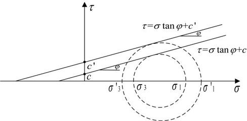
In Fig. 4, the cohesive strength parameter of soil ( $c$ ) under natural conditions is obtained when the soil micro-element is in the limit equilibrium state. Similarly, the ultimate cohesive strength parameter under the action of earthquake ( $c'$ ) is solved when the soil micro-element is in the limit equilibrium state under the action of earthquake. Through indoor shaking table tests under different accelerations, and combining with the direct shear tests of the soil before and after the earthquake, the shear strength parameters of the soil under different acceleration loads are obtained. The results show that the cohesion strength of soil decreases with the increase of peak acceleration, and the internal friction angle of soil slightly decreases [19]. Therefore, on this basis, assuming that the internal friction angle of the soil body ( $φ$ ) remains unchanged under the action of earthquake. By comparing Eq. (10) and Eq. (19), it can be found that $c'$ is greater than $c$ , which indicating that the stress circle of the slope micro-element under the action of earthquake $(τ = c' + σ t a n φ)$ is located above the action curve of stress circle without earthquake ( $τ = c + σ t a n φ$ ), and they are in a state of separation, which indicates that the stress state of a point on the slope sliding surface under the action of earthquake changes from critical stable state to failure state. The difference between the two cohesive forces is the cohesive force of soil to resist earthquake. At the same time, it can be proved that $k_{3} > k_{1}$ ( $∆ σ_{1} >$ 0), $k_{4} < k_{2}$ ( $∆ σ_{3} <$ 0), indicating that the stress circle becomes larger and moves to the right under the action of earthquake, and the slope stability decreases, as shown in Fig. 4.

Fig. 4Molar circle and strength envelope of slope soil under earthquake conditions

3.2.2. Simplified calculation model of slope stability

In this paper, the proportional coefficient of the cohesive strength of the slope with and without earthquake action is defined as $ε$ :

21

c^{'} = ε c .

According to Eq. (10) and Eq. (19), $ε$ can be written as:

22

ε = \frac{k_{3} - k_{4} - (k_{3} + k_{4}) s i n φ}{k_{1} - k_{2} - (k_{1} + k_{2}) s i n φ} .

Then the equivalent soil cohesive strength under the action of earthquake ( $c''$ ) is:

23

c^{''} = c - c^{'} + c = (2 - ε) c .

3.2.3. Calculation of slope stability coefficient

Based on the above simplified calculation model and method, $k_{1}$ , $k_{2}$ , $k_{3}$ , $k_{4}$ , $ε$ and the equivalent soil cohesion under the action of earthquake ( $c''$ ) are obtained according to Eq. (9), Eq. (18)-Eq. (23), as shown in Table 3.

In summary, the seismic action can be equivalent to the degradation effect of the initial cohesive strength of the soil. Geo-studio numerical simulation software and Lizheng geotechnical calculation software were used to automatically search for the most dangerous sliding surface to calculate the stability coefficient of the slope under the action of earthquake. The cohesive strength of the silty clay in the Geo-studio numerical simulation process adopts the natural cohesive strength of 30.2 kPa, and the cohesive strength of the silty clay in the calculation process of the Lizheng Geotechnical is calculated by Eq. (23), which is 12.68 kPa. The calculation results of stability coefficient of high cut slope are shown in Table 4. It can be seen that the numerical simulation result of Geo-Studio software is 1.167, and the Lizheng Geotechnical calculation results take the average of the three of 1.138, and the calculation results of Eq. (10) are 97.5 % of that of Geo-Studio numerical simulation. Considering the error of the numerical simulation process, there is no significant difference between them, indicating that the method is feasible and acceptable in engineering.

Table 3Calculation table of equivalent soil cohesion under earthquake action

$λ$	$Β$ (°)	$k_{1}$	$k_{2}$	$k_{3}$	$k_{4}$	$ε$	$c$ (kPa)	$c''$ (kPa)
0.67	45	0.92	–0.09	1.29	–0.17	1.58	30.20	12.68

Table 4Calculation table of high cut slope stability coefficient under earthquake action

Calculation software	Calculation method	Stability coefficient	Calculation software	Calculation method	Stability coefficient software
Geo-studio	Slope/W	1.167	Lizheng Geotechnical Calculation	Swedish Article Law	1.122
				Simplified Bishop method	1.147
				Janbu method	1.145

4. Numerical model of particle flow

4.1. Mesoscopic parameter calibration

In this paper, the micro parameters of silty clay and mudstone were calibrated by combining indoor triaxial test and PFC numerical triaxial servo test, on the premise that the stress-strain curves and shear strength indexes of the rock and soil samples obtained by them are relatively consistent, the micro parameters of rock and soil mass were determined.

In this paper, samples was obtained by on-site sampling, and the indoor triaxial test (CU) of silty clay was carried out by the TSZ-6A soil triaxial test instrument, as shown in Fig. 5(a). The parameters of the soil triaxial test instrument are shown in Table 5, the confining pressures adopted were 100 kPa, 200 kPa, 300 kPa, 400 kPa, and the corresponding PFC numerical triaxial servo test was shown in Fig. 5(c).

Fig. 5Indoor triaxial test and PFC numerical triaxial test of silty clay

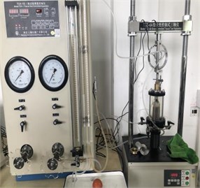
a) Indoor triaxial test

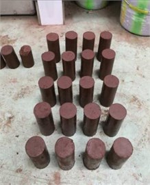
b) Sample of silty clay

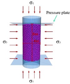
c) PFC numerical triaxial servo test

Table 5Parameters of soil triaxial tester

Specification model	Rated load	System confining pressure	Load rate	Back pressure	Volume change
TSZ-6A	3 kN	0-2 MPa	0.0024-4.5 mm/min	0.0024-0.8 MPa	0-50 ml

The mole failure envelopes obtained from the indoor triaxial test and PFC numerical triaxial servo test of silty clay are shown in Fig. 6 and Fig. 7, respectively.

Fig. 6Mole failure envelope of silty clay in indoor triaxial test

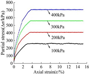
a) Stress-strain curve

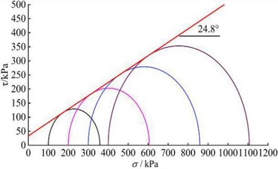
b) Mole failure envelope

Fig. 7Mole failure envelope of silty clay in numerical triaxial servo test

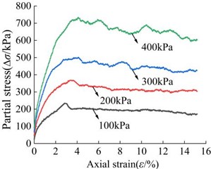
a) Stress-strain curve

b) Mole failure envelope

It can be seen that the cohesive strength of the silty clay ( $c$ ) is 32.8 kPa and the friction angle ( $φ$ ) is 23.7° obtained by the PFC triaxial servo test, which is close to the shear strength index of the silty clay sample in the indoor conventional triaxial test ( $c =$ 33.6 kPa, $φ =$ 24.8°), indicating that the micro parameters of silty clay calibrated by the PFC numerical triaxial servo test are more feasible, and the values of micro parameters of silty clay are finally determined in Table 7.

The indoor conventional triaxial test of mudstone samples was carried out on the RMT-150C rock mechanics test system, the parameters of the rock triaxial test instrument are shown in Table 6, the confining pressures adopted are 2 MPa, 4 MPa, 6 MPa, 8 MPa, and the corresponding PFC numerical triaxial servo test was shown in Fig. 8(c).

Table 6Parameters of rock triaxial tester

Maximum load	Vibration frequency	Maximum confining pressure	Confining pressure rate	Displacement measurement range	Strain measurement range
1000 kN	0.2-2 Hz	50 MPa	0.001-1 MPa/s	±50 mm	±0.01

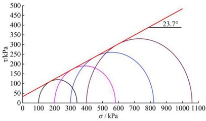
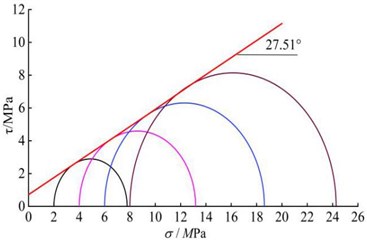
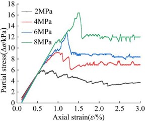
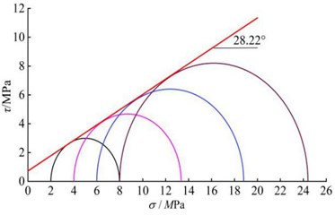
The mole failure envelopes obtained from the indoor triaxial test and PFC numerical triaxial servo test of mudstone are shown in Fig. 9 and Fig. 10, respectively.

In summary, the cohesive strength of the mudstone sample is 721.15 kPa and the internal friction angle is 28.22° obtained by the PFC triaxial servo test, which is close to the shear strength index of the mudstone sample in the indoor conventional triaxial test ( $c =$ 716.42 kPa, $φ =$ 27.51°), indicating that the mudstone micro parameters calibrated by the PFC numerical triaxial servo test can better simulate the mechanical properties of mudstone, and the values of micro parameters of silty clay are finally determined in Table 7.

Fig. 8Indoor triaxial test and PFC numerical triaxial servo test of mudstone

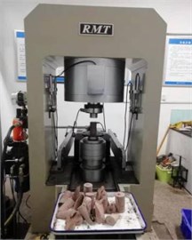
a) Indoor triaxial test

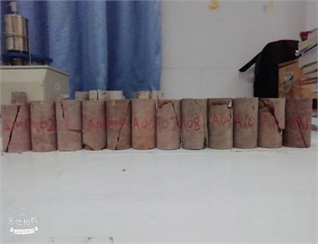
b) Sample of mudstone

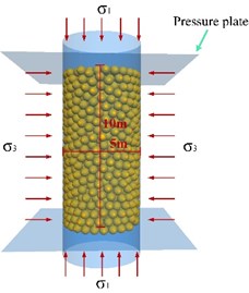
c) PFC numerical triaxial servo test

Fig. 9Mole failure envelope of mudstone in indoor triaxial test

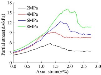
a) Stress-strain curve

b) Mole failure envelope

Fig. 10Mole failure envelope of mudstone in numerical triaxial servo test

a) Stress-strain curve

b) Stress-strain curve

4.2. Model building

4.2.1. Steps for building numerical model

The general process of establishing and solving PFC numerical model roughly includes four processes.

(1) Firstly, a model area needs to be defined. The size of the area is determined according to the actual calculated wall range, which is larger than the area occupied by the wall.

(2) Secondly, the walls and particles are built in the area. The size, number and distribution of particles are determined according to the actual engineering and calculation conditions.

(3) Thirdly, the particle constitutive model and related parameters are given, and the initial calculation is carried out to make the model reach the initial equilibrium state.

(4) Finally, the boundary and initial conditions are imposed to the model to simulate the related problems.

Table 7Mesoscopic parameters of particle flow model

	Parameter
Category	$d_{m i n}$ / mm Mm	$d_{m a x}$ / mm	$ρ$	$E$ / Mpa	$k^{*}$	$μ$	$\bar{E}$	${\bar{k}}^{*}$	${\bar{σ}}_{c}$ / Mpa	$\bar{c}$ / Mpa	$\bar{λ}$	$β_{n}$	$β_{s}$
Silty clay	0.2	0.22	1.85	300	1.5	0.85	0.3	1.5	0	1e3	1.0	1	1
Mudstone	0.35	0.36	2.5	100	1.3	1.2	10	1.3	4.2e6	4.2e6	1.01	1	1
$d_{m i n}$ – minimum particle size; $d_{m a x}$ – maximum particle size; $ρ$ – the relative density of particles; $E$ – the contact modulus of the particle; $k^{}$ – the stiffness ratio of particles; $μ$ – coefficient of friction of particles; $\bar{E}$ – parallel bonding modulus; $k^{}$ – parallel bonding stiffness ratio; ${\bar{σ}}_{c}$ – parallel bonding tensile strength; $\bar{c}$ – parallel bonding cohesion; $\bar{λ}$ – parallel bonding radius multiplier; $β_{n}$ – normal critical damping ratio; $β_{s}$ – tangential critical damping ratio

4.2.2. Boundary conditions and monitoring plan

The three-dimensional particle flow model of high cut slope was established by using the discrete element software PFC3D, as shown in Fig. 11.

Fig. 11PFC numerical model of three-dimensional particle flow

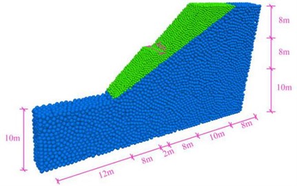
Fig. 12Boundary condition diagram of dynamic calculation and monitoring plan of the high cut slope

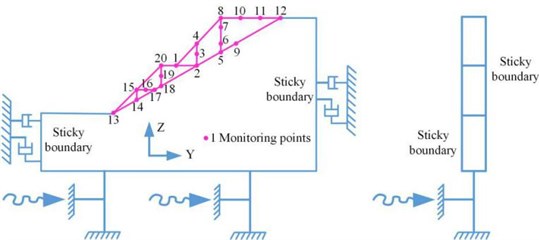
In this paper, seismic wave was applied to slope model by inputting time history curve of seismic wave acceleration at the bottom, and viscous boundary was used to prevent the reflection of input seismic wave at the boundary of the model, which can be achieved by setting dampers in the normal and tangential directions on both sides and the bottom boundary of the model, as shown in Fig. 12. At the same time, in order to obtain the time-frequency characteristics of high cut slope under the action of earthquake, 20 monitoring points were arranged along the slope surface, horizontal direction and vertical direction in the particle flow model to realize the real-time monitoring of the velocity parameters, as shown in Fig. 12.

4.3. Seismic waves

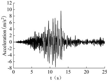
In the process of studying the influence of seismic forces on slope stability, the failure mode under the coupling of transverse and longitudinal waves has an amplifying effect on slope stability, the probability of both acting at the same point at the same time is small, and the actual effect is not large. Therefore, the first 25 s seismic waves of the E-W seismic time history record obtained at Wolong Station in the 2008 Wenchuan earthquake in Sichuan were adopted in this paper, and they were input into the bottom of the model as horizontal seismic waves. The acceleration time history curve is shown in Fig. 13.

Fig. 13Acceleration time history curve of seismic E-W wave

5. Dynamic response law

According to the above arrangement scheme of monitoring points, the law of time history of velocity, acceleration and displacement at the monitoring point within 25 s under the action of earthquake were obtained, and the dynamic response of high cut slope under the action of earthquake were studied. In order to describe the acceleration response law of the high cut slope under the action of earthquake in this paper, the PGA (Peak Ground Acceleration) amplification coefficient is used to indirectly analyze the peak acceleration, and the PGA amplification coefficient is defined as the ratio of peak acceleration of dynamic response of monitoring point to the peak acceleration of the input seismic wave (9.58 m/s²).

5.1. Dynamic response of the soil particles on slope surface

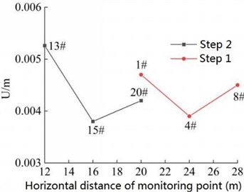
For the convenience of representation, monitoring point No. 1 is represented by monitoring point 1# in the process of data processing, and other monitoring points are similarly processed. Meanwhile, the lower left corner of the model is taken as the origin of coordinates (as shown in Fig. 12). During the period of seismic action, the distribution of velocity of the six monitoring points on the slope surface (as shown in Fig. 12) are shown in Fig. 14(a). In Fig. 14(b), the horizontal distance of the monitoring point refers to the horizontal distance between the monitoring point and the origin of coordinates in the lower left corner of the model. Step 1 refers to the upper step, step 2 refers to the lower step, and the following is similar. It can be found from Fig. 14 that for the monitoring points on the same step, the peak velocity of the foot of slope (monitoring point 1# and 13#) under the action of earthquake are greater than that of the slope shoulder (monitoring point 8# and 20#), and the monitoring points in the middle of the slope (monitoring point 4# and 15#) are the smallest, and the peak velocity and peak combined velocity in $Z$ and $Y$ directions of the monitoring point 13# on the slope 2 and monitoring point 8# on step 1 are significantly higher than the other monitoring points. It shows that the potential damage of the foot and shoulder of the high cut slope is more serious under the action of earthquake. The reason is that the shear stress concentration area of the silty clay slope is formed due to the cutting of the slope. Under the action of earthquake, the potential sliding signs of the lower part of high cut slope are more obvious, and shear deformation and failure are more likely to occur. The slope shoulder is located at the combination of the top and surface of the slope, where the tensile stress is concentrated, and the amplification effect of the seismic waves on the free surface is more obvious. It shows that the potential failure mode of the slope under the action of earthquake should start from the plastic failure at the foot of the slope, and develop upward to form the potential failure surface with the potential tensile crack at the slope top (caused by tensile stress), and then failure occurs.

Fig. 14Combined velocity of the monitoring point on slope surface

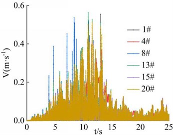
a) Time-history curve

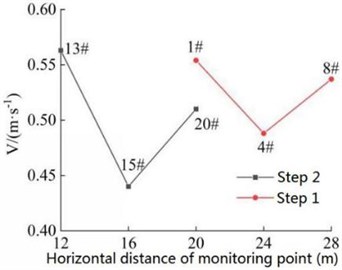
b) Peak distribution

Fig. 15Combined PGA amplification coefficient of the monitoring point on the slope surface

a) Time-history curve

b) Peak distribution

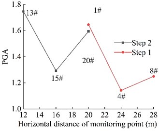
Fig. 15 shows the distribution of PGA amplification coefficient of the 6 monitoring points on the surface of high cut slope under the action of earthquake. It can be seen that the basic law is similar to the distribution of soil particles velocity. The PGA amplification coefficient of slope foot (monitoring point 1# and 13#) is larger than that of slope shoulder (monitoring point 8# and 20#) under the action of earthquake. The monitoring points in the middle of the high cut slope (monitoring point 4# and 15#) are the smallest, which means that the PGA amplification coefficient of the foot and shoulder of the high cut slope is greater than that of in the middle of the slope, and the PGA amplification coefficient of foot of step 2 is the largest. It shows that the dynamic response of slope foot and slope shoulder under the action of earthquake is more significant than that in the middle of the slope, and the slope foot is the most significant. It is suggested that reasonable excavation of the slope foot and the slope shoulder should be paid attention to during the excavation of natural slope.

The distribution of the displacements of the 6 monitoring points on the surface of the cut slope during the earthquake action period is shown in Fig. 16. It can be seen that the displacement of the monitoring points fluctuates with the magnitude of the seismic wave during the earthquake action period, and finally tends to be stable with the extension of earthquake action period. The main time node is the maximum acceleration time node of seismic wave, which is about 13 s under the action of seismic wave in this paper. Similar to the distribution of velocity and PGA amplification coefficient of the soil particles, the distribution of displacement of slope foot (monitoring point 1# and 13#) is larger than that of the slope shoulder (monitoring point 8# and 20#), and the displacement of monitoring points in the middle of slope (monitoring point 4# and 15#) is the smallest. The results show that the displacement of the foot and shoulder of the high cut slope is greater than that of the middle of the slope, and the monitoring point 13# at the foot of step 2 was most severely affected by seismic waves, and its final displacement is the largest.

Fig. 16Combined displacement of the monitoring point on slope surface

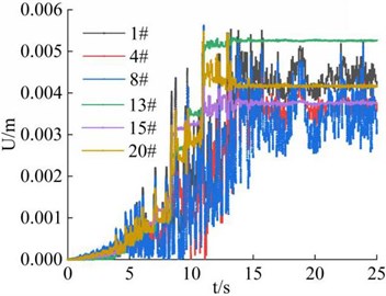
a) Time-history curve

b) Peak distribution

5.2. Dynamic response of the soil particles in the horizontal direction of the slope

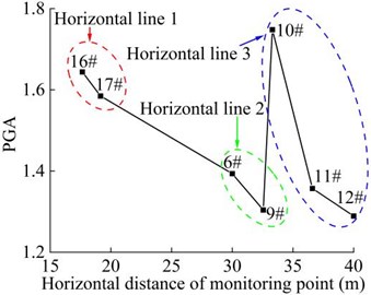
The distribution of velocity of the 7 monitoring points (as shown in Fig. 12) in the horizontal direction of the high cut slope during the earthquake action period is shown in Fig. 17. The 7 monitoring points constitute 3 horizontal lines. It can be seen that the monitoring point 9#, 12# and 17# on the three horizontal lines are located in the deepest part of the slope, and the monitoring point 6#, 10# and 16# are closest to the slope surface. In general, the velocity distribution of monitoring point 9#, 12# and 17# is less than that of monitoring point 6#, 10#, 11# and 16#, which shows that the closer the horizontal position is to the slope surface or away from the slope surface, the larger or smaller the peak values of velocity of each monitoring point in the horizontal direction, and the velocity distribution of each monitoring point is negatively correlated with the horizontal position. It can be seen that the dynamic response law of soil particles in horizontal direction under the action of earthquake is closely related to the distance from the surface of high cut slope.

Fig. 18 shows the distribution of PGA amplification coefficient of the 7 monitoring points in the horizontal direction under the action of earthquake. It can be seen that the PGA amplification coefficient of the monitoring point 9#, 12# and 17# in the innermost part of the slope has the lowest peak value, which is 1.304, 1.289 and 1.585, respectively. The PGA amplification coefficient of the monitoring point 6#, 10# and 16# in the outermost part of the slope has the highest peak value, which is 1.394, 1.748 and 1.644, respectively. The above phenomenon shows that the PGA amplification coefficient is closely related to the distance between the soil particles and the surface of the high cut slope. At the same height, as the horizontal position of the monitoring point is closer to the slope surface, the PGA amplification coefficient of the monitoring point shows a gradually increasing trend. In other words, at the same height, the amplification effect of slope of input ground motion on the slope surface is greater than that of the interior of slope, and free surface amplification effect appears, which shows a certain surface effect (surface-tending effect), which is caused by the reflection and superposition effect of the seismic wave on the free surface.

Fig. 17Combined velocity of the monitoring point in the horizontal direction

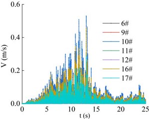
a) Time-history curve

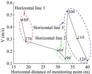
b) Peak distribution

Fig. 18Combined PGA amplification coefficient of the monitoring point in the horizontal direction

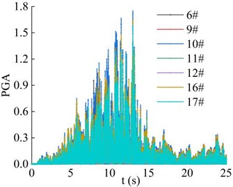
a) Time-history curve

b) Peak distribution

Fig. 19Combined displacement of the monitoring point in the horizontal direction

a) Time-history curve

b) Peak distribution

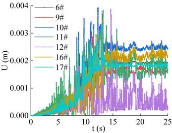
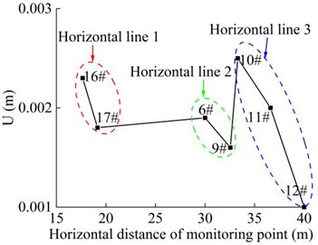
The distribution of displacements of the 7 monitoring points in the horizontal direction of the high cut slope during earthquake action period is shown in Fig. 19. It can be seen that the displacement of the monitoring points fluctuate with the magnitude of the seismic wave during the earthquake action period, and finally tended to be stable with the extension of the earthquake action period. The main time node is the maximum acceleration time node of seismic wave, which is about 13 s under the action of seismic wave in this paper. Similar to the distribution of velocity and PGA amplification coefficient of the soil particles, the distribution of displacement of monitoring point 16#, 6# and 10# is generally larger than that of monitoring point 17#, 9#, 11# and 12#. The results show that the closer to the slope surface, the larger the final values of the displacement of the monitoring points in the horizontal direction, showing the surface-tending effect or the free surface amplification effect, and the reason is the same as PGA amplification coefficient analysis. It is suggested that slope surface reinforcement measures should be implemented in time after the excavation of natural slope.

5.3. Dynamic response of the soil particles in the vertical direction of the slope

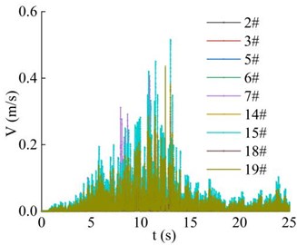
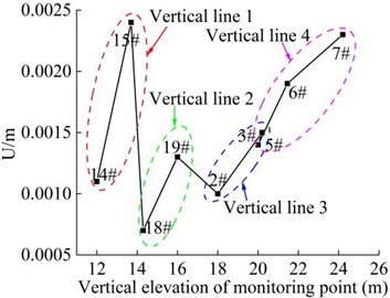
In Fig. 20, vertical elevation refers to the vertical distance between the monitoring points and the origin of coordinates in the lower left corner of the model. The distribution of velocity of the 9 monitoring points (as shown in Fig. 12) in the vertical direction of the high cut slope during earthquake action period is shown in Fig. 20. The 9 monitoring points constitute 4 vertical lines. It can be seen that the peak value of the velocity of the monitoring points with a lower elevation on each vertical line (monitoring point 14#, 18#, 2# and 5#) are all smaller than those of the monitoring points with a higher elevation (monitoring point 15#, 19#, 3#, 6# and 7#). It indicates that the peak velocity of monitoring points increases with the increase of elevation, showing an obvious velocity elevation amplification effect. At the same time, it can also be found that when the vertical elevation difference of the monitoring points on the vertical line 1 and the vertical line 2 of the step 2 is consistent, the difference of the velocity of the monitoring point 14# and 15# on the vertical line 1 is larger than that of monitoring point 18# and 19# on the vertical line 2. When the vertical elevation difference of the monitoring points on the vertical line 3 and the vertical line 4 of the step 1 is consistent, the difference of the velocity of the monitoring point 2# and 3# on the vertical line 3 is larger than that of monitoring point 5#, 6# and 7# on the vertical line 4. The results shows that the velocity amplification effect of slope on seismic wave decreases with the elevation, but does not increase indefinitely. This law is consistent with the conclusion found by wang when the homogeneous clay slope model was input into strong seismic waves [20].

Fig. 20Combined velocity of the monitoring point in the vertical direction

a) Time-history curve

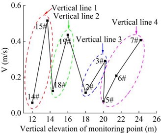
b) Peak distribution

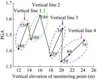
Fig. 21 shows the distribution of the PGA magnification coefficient of 9 monitoring points in the vertical direction under the action of earthquake. It can be seen that the basic law is similar to the distribution of soil particle velocity, which shows that the PGA magnification coefficient is closely related to the vertical elevation of soil particles. The PGA magnification coefficient is positively correlated with the vertical elevation of the soil particles. The PGA magnification coefficient of the monitoring point 14#, 18#, 2#, and 5# with the lower vertical elevation on the same vertical line is generally smaller than that of the monitoring points with higher elevation (monitoring points 15#, 19#, 3#, 6#, 7#). When the vertical elevation difference of the monitoring points on vertical line 1 and vertical line 2 of step 2 is consistent, difference of the PGA amplification coefficient of the monitoring point 14# and 15# on the vertical line 1 is greater than that of monitoring point 18# and 19# on the vertical line 2. When the vertical elevation difference of the monitoring points on the vertical line 3 and the vertical line 4 of the step 1 is consistent, the difference of the PGA amplification coefficient of the monitoring point 2# and 3# on the vertical line 3 is greater than that of monitoring point 5#, 6# and 7# on the vertical line 4. That is, the distribution of PGA amplification coefficient of the monitoring points in the vertical direction shows the PGA elevation amplification effect, but it is not infinite. This conclusion is consistent with the conclusion obtained by Xu and Yan in the model test of shaking surface that the PGA amplification coefficient increases with the increase of vertical elevation and shows an overall attenuation trend with the elevation, rather than an infinite increase [21, 22].

Fig. 21Combined PGA amplification coefficient of the monitoring point in the vertical direction

a) Time-history curve

b) Peak distribution

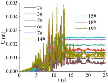
The distribution of the displacements of the 9 monitoring points in the vertical direction of the high cut slope during the earthquake action period is shown in Fig. 22. It can be seen that the displacements of the 9 monitoring points during the earthquake action period fluctuate with the magnitude of the seismic wave, and finally tended to be stable with the extension of the earthquake action period. The main time node is the maximum acceleration time node of seismic wave, which is about 13s under the action of seismic wave in this paper. In general, the law of the displacement value of the monitoring point is similar to that of the velocity and PGA magnification coefficient. The final displacement value of the monitoring point 14#, 18#, 2#, and 5# with lower vertical elevation on the same vertical line is generally smaller than that of the monitoring points with higher elevation (monitoring point 15#, 19#, 3#, 6#, 7#). When the vertical elevation difference of the monitoring points on vertical line 1 and vertical line 2 of step 2 is consistent, the difference of final displacement value of the monitoring point 14# and 15# on the vertical line 1 is greater than that of monitoring point 18# and 19# on the vertical line 2. When the vertical elevation difference of the monitoring points on the vertical line 3 and the vertical line 4 of the step 1 is consistent, the difference of the final displacement value of the monitoring point 2# and 3# on the vertical line 3 is greater than that of monitoring point 5#, 6# and 7# on the vertical line 4. The results shows that the displacement of the elevation amplification effect, that is, the peak displacement of each monitoring point in the vertical direction increases with the increase of elevation, and shows an overall attenuation trend with the elevation, rather than an infinite increase.

In summary, the velocity, PGA amplification coefficient, displacement and other characteristic quantities of the 20 monitoring points of the high cut slope were analyzed, it is found that the maximum displacement of the slope is located at the foot of the slope, about 5 mm, followed by the displacement of the slope shoulder. On the whole, the displacement of monitoring points on the slope surface is 3-5 mm, and the displacement of other monitoring points is 0-3 mm, which indicates that the displacement on the slope surface is greater than that of the interior part of the slope, and the displacement of the foot of slope is the largest. The potential failure mode of the slope should start from the shear failure of the slope foot and the tension failure of the slope shoulder, and then gradually penetrate. The above research shows that although the displacement of the slope occurs during the earthquake action period, the value is small. There is no obvious sign of sliding, and the slope is still in a stable state. This conclusion verifies the rationality of the simplified calculation method of the stability of high cut slope under the action of earthquake in Section 3.

Fig. 22Combined displacement of the monitoring point in the vertical direction

a) Time-history curve

b) Peak distribution

6. Time-frequency analysis of vibration signal of high cut slope

6.1. The basic principle

At present, the analysis object of vibration frequency is Fourier main frequency, which is based on the Fourier transform of a whole segment of signal, and the method commonly used to analyze the frequency spectrum of discrete sampling signals spectrum is the Fast Fourier Transform algorithm (FFT). Therefore, according to the acceleration time history curve of each monitoring point on the slope under the action of earthquake, MATLAB 2016a programming was adopted to transform (FFT) the acceleration time history signal of the monitoring point in this paper.

HHT (Hilbert-Huang Transform) is a new analysis method for processing nonlinear and non-stationary signals proposed by Huang E and Hilbert-Huang in 1998. It is a major breakthrough in linear and steady-state spectral analysis based on Fourier Transform in recent hundred years and currently widely used in seismic spectrum energy analysis [23]. Based on empirical mode decomposition (EMD), the signal is decomposed into the sum of a series of intrinsic mode functions (IMF), and then the instantaneous frequency is obtained by Hilbert transform (HHT) for each IMF [24].

The basic steps are as follows:

Firstly, EMD is used to decompose the complex signal into a finite number of intrinsic mode functions (IMF). Then, the cubic spline function is used to interpolate the extreme points on the original signal $x (t)$ , connect the envelopes fitted by the upper and lower extreme points, and define the mean value of the two envelopes as $m (t)$ , and subtract the original signal from the mean value to get:

24

y (t) = x (t) - m (t),

where, $x (t)$ is the original signal, $m (t)$ is the mean value of the upper and lower envelopes, $y (t)$ is the difference. Taking $y (t)$ as the original signal and repeating the above steps until the stopping criterion is satisfied after $n$ iterations, and the criterion is:

25

S D = {\sum_{t = 0}^{T} |\frac{y_{n - 1} (t) - y_{n} (t)}{y_{n - 1} (t)}|}^{2} .

Among them, the $S D$ value is generally between 0.2 and 0.3 to stop the iteration. At this time, $c_{1} = y_{1} (t)$ obtained after $n$ times of screening is the first IMF component. Then, the difference value between $x (t)$ and $c_{1} (t)$ is the new Signal, and the IMF components $c_{2}$ , $c_{3}$ ,..., $c_{n}$ can be obtained in turn. So far, the original signal can be decomposed into the sum of $n$ IMF components and the margin $r_{n}$ :

26

x (t) = \sum_{i = 1}^{n} c_{i} (t) + r_{n} (t),

where, $c (t)$ is the modal component, $r (t)$ is the residual margin.

2) Then, the Hilbert transform is performed on each IMF component to obtain the instantaneous frequency and amplitude of each IMF component $c (t)$ with time:

27

H [c (t)] = \frac{1}{π} P V \int_{- \infty}^{+ \infty} \frac{c (t^{'})}{t - t^{'}} d t^{'} .

where, $H$ is Hilbert spectrum; $P V$ is Cauchy principal value.

The analytical signal $z (t)$ is constructed as follows:

28

z (t) = c (t) + j H [c (t)] = a (t)^{'} e^{j φ (t)},

29

a (t) = \sqrt{c^{2} (t) + H^{2} [c (t)]},

30

Φ (t) = t a n^{- 1} \frac{H [c (t)]}{c (t)},

where, $a (t)$ is the amplitude function; $Φ (t)$ is the phase function.

Based on Eq. (30), the instantaneous frequency $f (t)$ is obtained, which is a function of time. It reflects a measure of the frequency concentration of the signal energy at a certain moment, that is, the instantaneous frequency of the signal. Its expression is as follows:

31

f (t) = \frac{1}{2 π} \frac{d Φ (t)}{d t} .

Hilbert transform each IMF component:

32

H (ω, t) = R E \sum_{i = 1}^{n} a_{i} (t) e^{\int ω_{i} (t) d t} .

The Hilbert spectrum, which reflects the joint distribution of “time-frequency-energy”, can be obtained by expressing the above formula as a function of three-dimensional time domain and frequency domain.

Hilbert instantaneous energy is defined as follows:

33

I E (t) = \int_{0}^{T} H^{2} (ω, t) d ω .

The instantaneous energy reflects the distribution of signal energy with time. The Hilbert energy spectrum can be obtained if the time is integrated by the square of the amplitude:

34

E S (ω) = \int_{0}^{T} H^{2} (ω, t) d t .

In order to study the distribution law of frequency band energy of seismic vibration, the frequency band energy analysis of seismic vibration signal can be carried out:

35

H (ω, t) = R E \sum_{i = 1}^{n} a_{i} (t) e^{\int ω_{i} (t) d t},

36

E^{'} (t) = \int_{- \infty}^{\infty} H^{' 2} (ω, t) d ω,

37

E (ω) = \int_{0}^{T} H^{2} (ω, t) d t,

where, $E (ω)$ is the marginal energy, which describes the distribution of signal energy with frequency. TE is the total energy of the signal based on the Hilbert transform. According to the sampling theorem [25], the Nyquist frequency is 250 Hz, that is, the highest frequency can be identified is 250 Hz since the sampling frequency is 500. In the process of wavelet packet analysis, the number of wavelet packet layers is set to 4, so 16 frequency bands are obtained, which are band 1, band 2,..., band 16, and the band degree of each frequency is 15.625 Hz, the frequency range of the frequency band is 0-15.625 Hz, 15.625-31.25 Hz,..., 234.375-250 Hz:

38

T E = \sum_{ω = 1}^{ω_{m a x}} E (ω) .

For the convenience of analysis, 125-250 Hz is defined as a high frequency band, collectively referred to as band 9. Namely, $e_{1}$ , $e_{2}$ , $e_{3}$ ,..., $e_{9}$ are set to the proportion of energy of band 1, band 2,..., band 9, respectively. The calculation formula is as shown in Eqs. (39-47):

39

e_{1} = \frac{\sum_{ω = 0}^{15.625} E (ω)}{T E},

40

e_{2} = \frac{\sum_{ω = 15.626}^{31.25} E (ω)}{T E},

41

e_{3} = \frac{\sum_{ω = 31.251}^{46.875} E (ω)}{T E},

42

e_{4} = \frac{\sum_{ω = 46.876}^{62.5} E (ω)}{T E},

43

e_{5} = \frac{\sum_{ω = 62.501}^{78.125} E (ω)}{T E},

44

e_{6} = \frac{\sum_{ω = 78.126}^{93.75} E (ω)}{T E},

45

e_{7} = \frac{\sum_{ω = 93.751}^{109.375} E (ω)}{T E},

46

e_{8} = \frac{\sum_{ω = 109.376}^{125} E (ω)}{T E},

47

e_{9} = \frac{\sum_{ω = 125.001}^{250} E (ω)}{T E} .

6.2. Results and discussion

6.2.1. Time-frequency analysis of monitoring points on the slope surface

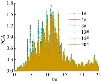
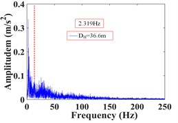
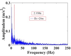
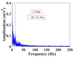
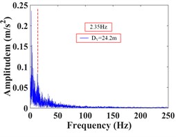
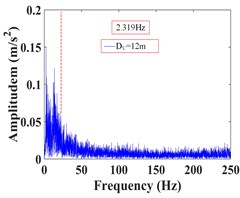
Based on Fourier transform, the frequency spectrum of each monitoring point of the slope is shown in Fig. 24, and the Fourier dominant frequency of each monitoring point was extracted, as shown in Fig. 25. The horizontal distance between the monitoring point and the origin of the model coordinates is represented by $D_{H}$ , and the vertical elevation of the monitoring point is represented by $D_{V}$ .

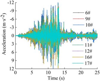
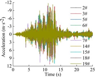
Fig. 23Acceleration of the monitoring points on the slope surface

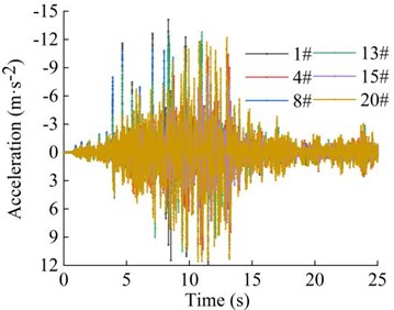
Fig. 24Acceleration spectrum diagram of the monitoring points on the slope surface

a) Monitoring point 1#

b) Monitoring point 4#

c) Monitoring point 8#

d) Monitoring point 13#

e) Monitoring point 15#

f) Monitoring point 20#

Table 8 shows the proportion of vibration frequency band energy of each monitoring point on the slope surface.

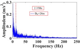
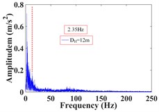
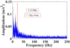
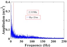
It can be seen that the vibration frequency of the monitoring point 1# at the foot of the upper step within 25 s of the earthquake action is mainly concentrated in 0-15 Hz, and the Fourier main frequency is 2.35 Hz. The vibration frequency of the monitoring point 8# at the shoulder of the slope is mainly concentrated in 0-20 Hz, and the Fourier main frequency is 2.35 Hz. The vibration frequency distribution of monitoring point 4# in the middle of the slope is relatively average, which is distributed within the maximum frequency, and the Fourier main Frequency is 18.31 Hz. The vibration frequency of the monitoring point 13# at the foot of the lower step within 25s of the earthquake action is mainly concentrated in 0-15 Hz, and the Fourier main frequency is 2.35 Hz. The vibration frequency of the monitoring point 20# at the shoulder of the slope is mainly concentrated in 0-20 Hz, and the Fourier main frequency is 2.319 Hz. The vibration frequency distribution of monitoring point 15# in the middle of the slope is mainly concentrated in 0-25 Hz, and the Fourier main Frequency is 2.319 Hz. The low frequency band (0-15.625 Hz) accounts for the largest proportion of frequency band energy of monitoring point 1# and 8# on the upper slope surface, and the high frequency band (125-250 Hz) only accounts for 2.38 % and 4.00 %. The energy of different frequency bands at monitoring point 4# in the middle of the slope is relatively uniform, and the high frequency band (125-250 Hz) accounted for 26.22 %. The low frequency band (0-15.625 Hz) accounts for the largest proportion of frequency band energy of monitoring point 13# and 20# on the lower slope surface, and the high frequency band (125-250 Hz) only accounts for 1.15 % and 4.47 %. The energy of different frequency bands at monitoring point 15# in the middle of the slope is relatively uniform, and the high frequency band (125-250 Hz) accounted for 9.32 %. It can be seen that the frequency band width in the middle of slope is larger than that in slope shoulder under the action of earthquake, and the slope foot is the smallest, and gradually develops towards low frequency, which indicates that the high frequency components in the slope shoulder and the middle part of the slope are larger than that in the slope foot, and the high frequency components in the middle of slope are the most, and the low frequency components in the slope foot are the most. The Fourier main frequency of each monitoring point is distributed between 0 and 5Hz (except for the monitoring point 4#), and the overall trend is that the dominant frequency in the middle of the slope is greater than that in the shoulder of the slope, and the minimum is at the foot of the slope.

Fig. 25Distribution diagram of Fourier dominant frequency of the monitoring points on the slope surface

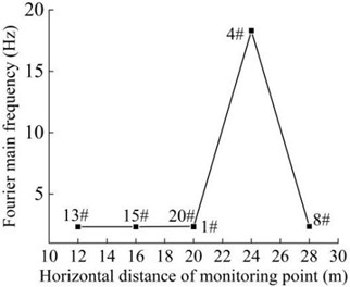
Table 8The proportion of frequency band energy of the monitoring points on the slope surface

Monitoring points	Frequency (Hz)
Monitoring points	0-15.625	15.625-31.25	31.25-46.875	46.87-62.5	62.5-78.125	78.125-93.75	93.75-109.375	109.375-125	125- 250
1#	76.05	9.71	2.60	4.48	0.42	1.02	1.70	1.64	2.38
4#	18.82	21.57	6.27	8.33	3.12	4.53	6.18	4.96	26.22
8#	67.69	11.76	3.98	4.74	0.99	1.75	3.09	2.00	4.00
13#	88.07	5.13	0.85	1.43	0.37	0.82	0.84	1.35	1.15
15#	47.90	23.23	4.03	7.75	1.21	1.71	2.71	2.13	9.32
20#	66.29	8.65	4.47	5.18	1.58	2.84	3.41	2.81	4.47

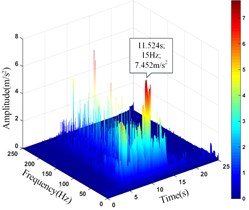
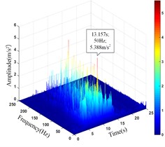
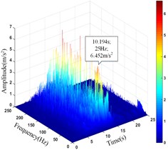
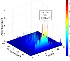
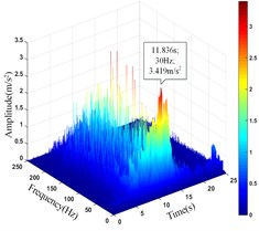
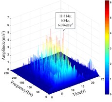
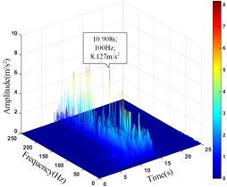
Based on the HHT transformation, the HHT three-dimensional time-frequency diagram (time-frequency-amplitude 3D diagram) of each monitoring point of the slope surface was obtained, as shown in Fig. 26.

The comparison results of the peak value ( $a_{m}$ ) and corresponding time ( $t_{a m}$ ) of the acceleration time history curve at each monitoring point in Fig. 23 and the amplitude main peak ( $A_{m}$ ) and corresponding time ( $T_{A m}$ ) of the HHT three-dimensional time-frequency diagram in Fig. 26 are shown in Table 9.

Fig. 26HHT three-dimensional time-frequency diagram of monitoring points on the slope surface

a) Monitoring point 1#

b) Monitoring point 4#

c) Monitoring point 8#

d) Monitoring point 13#

e) Monitoring point 15#

f) Monitoring point 20#

Table 9Comparison of am, tam, Am and TAm of the monitoring points on the slope surface

Monitoring points	Parameter
Monitoring points	$a_{m}$ (m/s²)	$t_{a m}$ (s)	$A_{m}$ (m/s²)	$T_{A m}$ (s)
1#	11.915	11.500	7.452	11.524
4#	10.392	13.100	5.388	13.157
8#	10.998	10.900	6.425	10.914
13#	11.172	13.200	7.304	13.288
15#	8.317	11.506	3.419	11.836
20#	10.178	11.523	6.076	11.814

It can be seen that the amplitude main peak of HHT three-dimensional time-frequency diagram at the monitoring point 1#, 4# and 8# on the upper step is 7.452 m/s², 5.388 m/s²and 6.425 m/s², respectively. The corresponding time is 11.524 s, 13.157 s and 10.914 s, respectively. The amplitude main peak of HHT three-dimensional time-frequency diagram at the monitoring point 13#, 15# and 20# on the lower step is 7.304 m/s², 3.419 m/s²and 6.076 m/s², respectively. The corresponding time is 13.288 s, 11.836 s and 11.814 s, respectively. Comparing the peak value of acceleration time-history curve and the corresponding time of the monitoring points, it can be found that the amplitude main peak at the foot of the slope is larger than that at the slope shoulder and the smallest in the middle of the slope, which is consistent with the distribution law of acceleration, and the corresponding time of the two peaks is relatively consistent, indicating the rationality and superiority of using HHT three-dimensional time-frequency analysis to analyze the dynamic response of high cut slope under the action of earthquake.

6.2.2. Time-frequency analysis of monitoring points in the horizontal direction

The analysis steps of the time-frequency analysis of the velocity signal of each monitoring point in the horizontal direction are the same as the monitoring point of the slope surface, as follows.

Fig. 27Acceleration of the monitoring points in the horizontal direction

a) The time history curve

b) Peak distribution

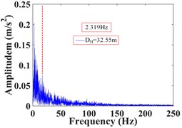
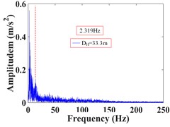
Fig. 28Acceleration spectrum diagram of the monitoring points in the horizontal direction

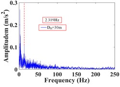
a) Monitoring point 6#

b) Monitoring point 9#

c) Monitoring point 10#

d) Monitoring point 11#

e) Monitoring point 12#

f) Monitoring point 16#

g) Monitoring point 17#

Table 10 shows the proportion of vibration frequency band energy of each monitoring point in the horizontal direction.

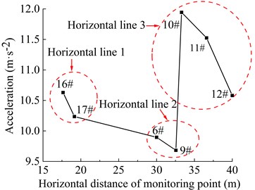
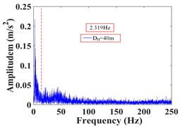
As can be seen from Fig. 28, the frequency of monitoring point 16# and 17# on horizontal line 1 within 25 s of earthquake action is mainly concentrated in 0-15 Hz and 0-35 Hz, respectively. The Fourier main frequency is 2.319 Hz and 3.174 Hz, respectively. Among them, the frequency distribution of monitoring point 17# is relatively uniform, with a large proportion in the maximum frequency. The frequency of the monitoring point 6# and 9# on horizontal line 2 is mainly concentrated in 0-10 Hz and 0-20 Hz, respectively, and the Fourier main frequency is 2.319 Hz. The frequency of the monitoring point 10#, 11# and 12# on horizontal line 3 is mainly concentrated in 0-10 Hz, 0-15 Hz and 0-20 Hz, respectively, and the Fourier main frequency is 2.319 Hz. The Fourier main frequency of each monitoring point is mainly concentrated in 0-5 Hz. It can be found from Table 10 that the frequency band energy of monitoring point 16# on horizontal line 1 accounts for the largest proportion of 0-15.625 Hz, while the high frequency band (125-250 Hz) only accounts 3.89 %, the frequency band energy of monitoring point 17# accounts for the largest proportion of 0-31.25 Hz, and the high frequency band (125-250 Hz) accounts for 8.95 %. Among them, monitoring point 16# is closer to the slope surface than monitoring point 17#. On the horizontal line 2, the frequency band energy of monitoring point 6# and 9# accounts for 80.86 % and 71.81 % in the frequency band of 0-15.625 Hz, respectively. The high frequency band (125-250 Hz) accounts for 2.35 % and 3.33 %, respectively. Among them, monitoring point 6# is closer to the slope surface than monitoring point 9#. On the horizontal line 3, the frequency band energy of monitoring point 10#, 11# and 12# accounts for 81.16 %, 59.59 % and 51.80 % in the frequency band of 0-15.625 Hz, respectively. The high frequency band (125-250 Hz) accounts for 1.82 %, 2.38 % and 12.15 %, respectively. Among them, monitoring point 10# is closer to the slope surface than monitoring point 11#, and monitoring point 12# is located at the deepest inside the slope.

Fig. 29Distribution diagram of Fourier dominant frequency of the monitoring points in the horizontal direction

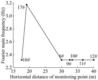
Table 10The proportion of frequency band energy of the monitoring points in the horizontal direction

Monitoring points		Frequency (Hz)
Monitoring points		0-15.625	15.625-31.25	31.25-46.875	46.875-62.5	62.5-78.125	78.125-93.75	93.75-109.375	109.375-125	125- 250
Horizontal line 2	6#	80.86	10.03	1.39	2.73	0.39	0.46	0.99	0.80	2.35
Horizontal line 2	9#	71.81	12.15	2.78	6.30	0.35	0.70	1.32	1.27	3.33
Horizontal line 3	10#	81.16	6.52	1.92	3.81	0.84	0.89	1.68	1.36	1.82
	11#	59.59	16.76	3.99	10.50	0.70	1.21	2.40	2.45	2.38
	12#	51.80	8.05	6.42	11.86	1.69	1.87	3.08	3.07	12.15
Horizontal line 1	16#	60.28	14.97	4.50	10.46	0.66	0.91	2.79	1.54	3.89
Horizontal line 1	17#	32.52	27.13	6.49	10.88	2.23	2.52	5.07	4.21	8.95

It can be seen that the distribution of low frequency band of each monitoring point on the high cut slope increases with the horizontal position of the monitoring point closer the slope surface under the action of earthquake, that is, the closer the horizontal position is to the slope surface, the more low frequency components and the less high frequency components, the distribution of low frequency band of the monitoring points is negatively correlated with the horizontal position. The above phenomenon show that the silty clay high cut slope has a filtering effect on the frequency spectrum components of the input seismic wave, and the high frequency components in the input seismic waves are filtered out. Moreover, the closer the horizontal position of soil particles is to the slope surface, the stronger the filtering effect of the slope on the high frequency band.

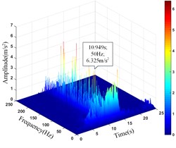
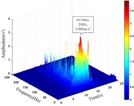
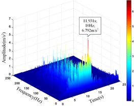
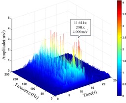
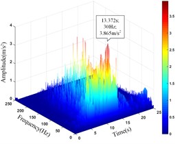
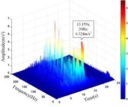
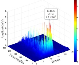
Based on the HHT transformation, the HHT three-dimensional time-frequency diagram (time-frequency-amplitude 3D diagram) of each monitoring point in the horizontal direction was obtained, as shown in Fig. 30.

Fig. 30HHT three-dimensional time-frequency diagram of monitoring points in the horizontal direction

a) Monitoring point 6#

b) Monitoring point 9#

c) Monitoring point 10#

d) Monitoring point 11#

e) Monitoring point 12#

f) Monitoring point 16#

g) Monitoring point 17#

The comparison results of the peak value ( $a_{m}$ ) and corresponding time ( $t_{a m}$ ) of the acceleration time history curve at each monitoring point in Fig. 27 and the amplitude main peak ( $A_{m}$ ) and corresponding time ( $T_{A m}$ ) of the HHT three-dimensional time-frequency diagram in Fig. 30 are shown in Table 11.

Table 11Comparison of am, tam, Am and TAm of the monitoring points in the horizontal direction

Monitoring points	Parameter
Monitoring points	$a_{m}$ (m/s²)	$t_{a m}$ (s)	$A_{m}$ (m/s²)	$T_{A m}$ (s)
6#	9.711	10.888	6.325	10.949
9#	9.683	10.898	3.880	10.946
10#	11.897	11.518	6.972	11.931
11#	11.525	13.082	4.000	11.614
12#	10.581	13.198	3.865	13.372
16#	11.749	13.072	6.324	13.159
17#	10.847	13.012	5.643	13.122

It can be seen that the amplitude main peak of HHT three-dimensional time-frequency diagram at the monitoring point 16# and 17# on horizontal line 1 under the action of earthquake is 6.324 m/s²and 5.643 m/s², respectively. The peak value of the time-history curve of acceleration is 11.749 m/s²and 10.847 m/s², respectively. The amplitude main peak of HHT three-dimensional time-frequency diagram at the monitoring point 6# and 9# on horizontal line 2 is 6.325 m/s²and 3.880 m/s², respectively. The peak value of the time-history curve of acceleration is 9.711 m/s²and 9.683 m/s², respectively. The amplitude main peak of HHT three-dimensional time-frequency diagram at the monitoring point 10#, 11# and 12# on horizontal line 3 is 9.762 m/s², 4.000 m/s²and 3.865 m/s², respectively. The peak value of the time-history curve of acceleration is 11.897 m/s², 11.525 m/s²and 10.581 m/s², respectively. Comparing the peak value of the history curve and the acceleration time of the monitoring points, it can be found that the innermost monitoring point 17#, 9# and 12# have the smallest amplitude main peaks, and the outermost monitoring point 16#, 6# and 10# have the largest amplitude main peaks. The amplitude main peaks of the monitoring points on the horizontal line at the same height increase with the horizontal position of the monitoring point closer the slope surface, which is consistent with the distribution law of acceleration, and the corresponding time of the them is close to the same, indicating the rationality and superiority of using HHT three-dimensional time-frequency analysis to analyze the dynamic response of high cut slope under the action of earthquake.

6.2.3. Time-frequency analysis of monitoring points in the vertical direction

The analysis steps of the time-frequency analysis of the velocity signal of each monitoring point in the horizontal direction are the same as the monitoring point of the slope surface, as follows.

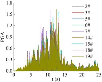
Fig. 31Acceleration of the monitoring points in the vertical direction

a) The time history curve

b) Peak distribution

Table 12 shows the proportion of vibration frequency band energy of each monitoring point in the vertical direction.

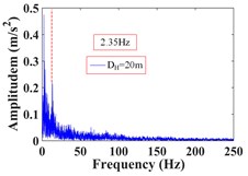
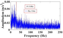
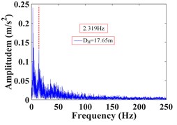
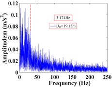
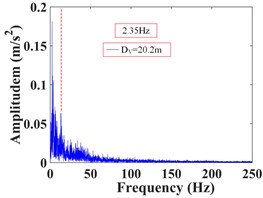
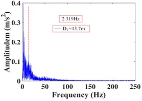
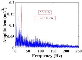
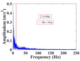
As can be seen from Fig. 32, the frequency of monitoring point 2# and 3# on the vertical line 3 of the upper step under the action of the earthquake are mainly concentrated in 0-20 Hz and 0-15 Hz, respectively. The Fourier main frequency is 2.35 Hz. The frequency of monitoring point 5#, 6# and 7# on the vertical line 4 of the upper step are mainly concentrated in 0-15 Hz, and the Fourier main frequency is 2.35 Hz. The frequency of monitoring point 14# and 15# on the vertical line 1 of the lower step under the action of the earthquake are mainly concentrated in 0-25 Hz and 0-15 Hz, respectively. The Fourier main frequency is 2.319 Hz. The frequency of monitoring point 18# and 19# on the vertical line 2 of the upper step are mainly concentrated in 0-25 Hz and 0-15 Hz, and the Fourier main frequency is 2.319 Hz, among them, the frequency distribution of monitoring point 18# is relatively uniform, with a large proportion in the maximum frequency. It can be found from Table 12 that the frequency band energy of monitoring point 2# on horizontal line 3 of the upper step accounts the largest proportion of 0-31.25 Hz, the high frequency band (125-250 Hz) only accounts 1.37 %, the frequency band energy of monitoring point 3# accounts the largest proportion of 0-15.625 Hz, and the rest frequency bands account for a relatively small proportion. The frequency band energy of monitoring point 5#, 6#, 7# on horizontal line 4 of the upper step accounts for 60.13 %, 80.86 % and 82.19 % of the frequency band of 0-15.625 Hz, indicating that the distribution of low frequency band of each monitoring point of the upper step on the high cut slope increases with the increase of its elevation, that is, the higher the elevation, the more low frequency components and the less high frequency components. The frequency band energy of monitoring point 14# on horizontal line 1 of the lower step accounts the largest proportion of 0-31.25 Hz, the high frequency band (125-250 Hz) accounts 9.29 %. The frequency band energy of monitoring point 15# on horizontal line 1 of the lower step accounts the largest proportion 0-15.625 Hz, the high frequency band (125-250 Hz) only accounts 0.34 %. The frequency band energy of monitoring point 19# on horizontal line 2 of the lower step accounts the largest proportion of 0-15.625 Hz, the high frequency band (125-250 Hz) only accounts 9.29 %. In contrast, the distribution of frequency band of monitoring point 18# is relatively uniform, and the high frequency band accounts for 10.74 %. The results shows that the distribution of low frequency band of each monitoring point of the lower step of high cut slope is positively correlated with its elevation, which is the same as the response characteristic of the monitoring points of the upper step. The above phenomenon indicate that the silty clay high cut slope has a filtering effect on the frequency spectrum components of the input seismic wave, and the high frequency components in the input seismic waves are filtered out. Moreover, the higher the vertical elevation of soil particles, the stronger the filtering effect of the slope on the high frequency band.

Fig. 32Acceleration spectrum diagram of the monitoring points in the vertical direction

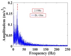
a) Monitoring point 2#

b) Monitoring point 3#

c) Monitoring point 5#

d) Monitoring point 6#

e) Monitoring point 7#

f) Monitoring point 14#

g) Monitoring point 15#

h) Monitoring point 18#

i) Monitoring point 19#

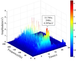
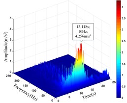
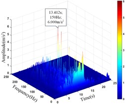
Based on the HHT transformation, the HHT three-dimensional time-frequency diagram (time-frequency-amplitude 3D diagram) of each monitoring point in the vertical direction was obtained, as shown in Fig. 34.

The comparison results of the peak value ( $a_{m}$ ) and corresponding time ( $t_{a m}$ ) of the acceleration time history curve at each monitoring point in Fig. 31 and the amplitude main peak ( $A_{m}$ ) and corresponding time ( $T_{A m}$ ) of the HHT three-dimensional time-frequency diagram in Fig. 34 are shown in Table 13.

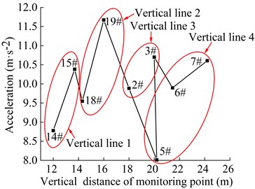
Fig. 33Distribution diagram of Fourier dominant frequency of the monitoring points in the vertical direction

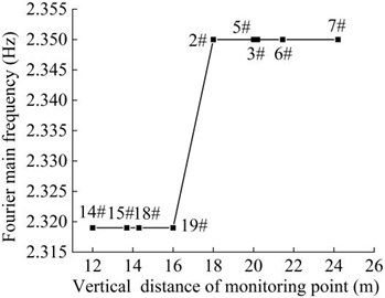
Table 12The proportion of frequency band energy of the monitoring points in the vertical direction

Monitoring points		Frequency (Hz)
Monitoring points		0-15.625	15.625-31.25	31.25-46.875	46.875-62.5	62.5-78.125	78.125-93.75	93.75-109.375	109.375-125	125-250
Vertical line 3	2#	44.00	39.06	2.13	10.05	0.31	0.45	1.79	0.86	1.37
Vertical line 3	3#	78.77	10.16	1.66	6.36	0.28	0.39	0.90	0.63	0.85
Vertical line 4	5#	60.13	10.62	4.78	9.52	1.65	1.64	3.22	2.06	6.37
	6#	80.86	10.03	1.39	2.73	0.39	0.46	0.99	0.80	2.35
	7#	82.19	10.33	1.05	4.11	0.16	0.24	0.93	0.43	0.57
Vertical line 1	14#	47.95	23.21	4.02	7.77	1.20	1.72	2.71	2.13	9.29
Vertical line 1	15#	83.05	12.98	0.94	1.70	0.06	0.10	0.59	0.24	0.34
Vertical line 2	18#	30.49	22.02	6.26	10.67	3.16	4.59	5.12	6.96	10.74
Vertical line 2	19#	84.61	6.07	1.71	3.60	0.27	0.39	1.03	0.93	1.29

Table 13Comparison of am, tam, Am and TAm of the monitoring points in the vertical direction

Monitoring points	Parameter
Monitoring points	$a_{m}$ (m/s²)	$t_{a m}$ (s)	$A_{m}$ (m/s²)	$T_{A m}$ (s)
2#	9.770	10.908	2.316	10.926
3#	11.241	11.536	6.647	11.550
5#	8.013	10.904	2.913	10.925
6#	9.711	10.888	6.325	10.941
7#	10.906	11.506	8.127	11.636
14#	10.311	11.538	4.185	11.546
15#	10.383	13.016	4.256	13.118
18#	9.549	13.026	6.000	13.145
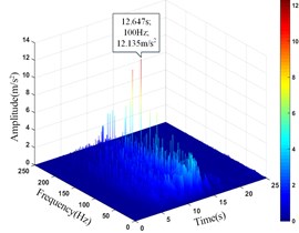
19#	11.057	12.492	12.135	12.647

Comparing the peak value of the acceleration time history curve of the monitoring points, it can be seen from Table 13 that the amplitude main peak of the monitoring points on the same vertical line increases with the elevation, which is consistent with the distribution law of acceleration, and the corresponding time of them is close to the same, indicating the rationality and superiority of using HHT three-dimensional time-frequency analysis to analyze the dynamic response of high cut slope under the action of earthquake. At the same time, it can also be found from the vertical line 4 that the difference between the main peaks of the monitoring point 5# and 6# is greater than that between the monitoring point 6# and 7#, which also shows that although the amplitude main peak of the monitoring points show an increasing trend with its elevation as a whole, the increasing trend gradually decays instead of increasing infinitely.

Fig. 34HHT three-dimensional time-frequency diagram of monitoring points in the vertical direction

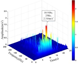
a) Monitoring point 2#

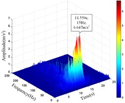
b) Monitoring point 3#

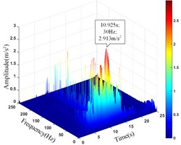
c) Monitoring point 5#

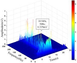
d) Monitoring point 6#

e) Monitoring point 7#

f) Monitoring point 14#

g) Monitoring point 15#

h) Monitoring point 18#

i) Monitoring point 19#

7. Conclusions

Based on the theoretical calculation and PFC3D numerical simulation method, the dynamic response law and time-frequency characteristics of high cut slope under the action of earthquake were studied. The following conclusions can be drawn from this study:

1) Under the action of earthquake, the width of frequency band of the soil particles in the middle of the slope is larger than that of the slope shoulder, the slope foot is the smallest, and gradually develops towards low frequency. The high frequency component in the middle of slope is the most, and the low frequency component in the foot of slope is the most.

2) Under the action of earthquake, the distribution of low frequency band of soil particles in the horizontal direction increases as its horizontal position is closer to the slope surface. The closer the horizontal position is to the slope surface, the more low the frequency components, which shows a certain surface-tending effect.

3) Under the action of earthquake, the distribution of low frequency band of soil particles in the vertical direction increases with its elevation, the higher the elevation, the more low frequency components, and the distribution of low frequency band is positively correlated with the elevation, which shows a certain elevation amplification effect.

4) Under the action of earthquake, the Fourier main frequency of soil particles is distributed between 0-5 Hz, and the frequency is mainly distributed in the low frequency band (0-15.625 Hz). The low frequency band accounts for 88.07 %, and the high frequency band (125-250 Hz) accounts for only 0.34 %, indicating that the dynamic response of high cut slope under the action of earthquake should focus on the influence of low frequency band on the stability of high cut slope.

References

Meei Ling Lin, Kuo Lung Wang Seismic slope behavior in a large-scale shaking table model test. Engineering Geology, Vol. 11, Issue 1, 2016, p. 118-133.

Publisher
Giri D., Sengupta A. Dynamic behavior of small-scale model slopes in shaking table tests. International Journal of Geotechnical Engineering, Vol. 4, Issue 1, 2014, p. 1-11.

Publisher
You A. F., Kong J. M., Ni Z. Q. Research the excavation angle affect on seismic dynamic response of slope. Advanced Materials Research, Vol. 374, Issue 2011, 2012, p. 2583-2587.

Publisher
Zhang J. W. Seismic Dynamic Response Analysis and Stability Evaluation Soil Slope. China Earthquake Administration, Beijing, 2015.

Search CrossRef
Tang H. Seismic Response and Dynamic Failure Mechanism Research on Layered Soil Slope. Southwest Jiaotong University, Sichuan, 2016.

Search CrossRef
Zhang J. W., Li X. J., Yuan Y., et al. Influence law of ground motion parameters. Acta Seismologica Sinica, Vol. 39, Issue 1, 2017, p. 798-805.

Search CrossRef
Deng T. X. Research on Dynamic Response Rules and Failure Mechanism of Alternatively Distributed Soft and Hard Bedding Slopes under Strong Earthquake. Southwest Jiaotong University, Sichuan, 2018.

Search CrossRef
Zhao J., Wu H. G., Yang T. Dynamic response of landslides to different seismic wave. The Chinese Journal of Geological Hazard and Control, Vol. 29, Issue 1, 2018, p. 47-52.

Search CrossRef
Yan Z., Zhang S., Zhang X., et al. Dynamic response law of loess slope with different shapes. Advances in Materials Science and Engineering, Vol. 1, Issue 2019, 2019, p. 4853102.

Publisher
Chen J. C., Wang L. M., Wang P., et al. Dynamic response of loess slopes based on the shake table test. China Earthquake Engineering Journal, Vol. 42, Issue 1, 2020, p. 529-535.

Search CrossRef
Yang C. W., Zhang J. J., J. W. Application of Hilbert-Huang Transform to the analysis of the landslides triggered by the Wenchuan earthquake. Journal of Mountain Science, Vol. 12, Issue 1, 2015, p. 711-720.

Publisher
Fan G., Zhang L. M., Zhang J. J., et al. Energy-based analysis of mechanisms of earthquake-induced landslide using Hilbert-Huang transform and marginal spectrum. Rock Mechanics and Rock Engineering, Vol. 50, Issue 1, 2017, p. 2425-2441.

Publisher
Fan G., Zhang L. M., Zhang J. J., et al. Analysis of seismic stability of an obsequent rock slope using time-frequency method. Rock Mechanics and Rock Engineering, Vol. 52, Issue 1, 2019, p. 3809-3823.

Publisher
Song D. P., Chen Z., Chao H., et al. Numerical study on seismic response of a rock slope with discontinuities based on the time-frequency joint analysis method. Soil Dynamics and Earthquake Engineering, Vol. 133, Issue 1, 2020, p. 106112.

Publisher
Xu Z. L. A Concise Course of Elastic Mechanics. Higher Education Press, Beijing, 1983.

Search CrossRef
Liu C. H., Chen C. G., Feng X. T. Study on the mechanism of slope instability induced by reservoir water level rise. Rock and Soil Mechanics, Vol. 26, Issue 5, 2005, p. 769-773.

Search CrossRef
Li G. X., Zhang B. Y., Yu Y. Z., et al. Soil Mechanics. Tsinghua University Press, Beijing, 2017.

Search CrossRef
Zhu Q. P. Improvement of Quasi-Static Method for Slope Seismic Stability Analysis. Chongqing University, Chongqing, 2015.

Search CrossRef
Ai H., Wu H. G., Yang T., et al. Experimental study on shear strength parameters of soil after earthquake. Chinese Science and Technology Papers, Vol. 11, Issue 13, 2016, p. 1544-1547.

Search CrossRef
Wang R. M. Experimental Study on Dynamic Response and Failure Mode of Different Soil Slopes under Earthquake Action. Southwest Jiaotong University, Sichuan, 2016.

Search CrossRef
Xu G. X. Research on the Dynamic Responses and Permanent Displacement of Slope under Earthquake. Southwest Jiaotong University, Sichuan, 2011.

Search CrossRef
Yan Z. X., Zhang L. P., Cao X. H., et al. Dynamic response law and deformation mechanism of bedding rock slope under earthquake. Chinese Journal of Geotechnical Engineering, Vol. 33, Issue 1, 2011, p. 61-65.

Search CrossRef
Huang N. E., Shen Z., Long S. R., et al. The empirical mode decomposition and the Hilbert spectrum for nonlinear and non-stationary time series analysis. Proceedings Mathematical Physical and Engineering Sciences, Vol. 454, Issue 1, 1998, p. 903-995.

Publisher
Zhang Y. P. HHT Analysis and Application Research of Blasting Vibration Signal. Central South University, Changsha, 2006.

Search CrossRef
Wang D. L. Digital Signal Processing. Tsinghua University Press, Beijing, 2014.

Search CrossRef

About this article

Received

25 October 2020

Accepted

27 January 2021

Published

19 February 2021

SUBJECTS

Seismic engineering and applications

DOI

https://doi.org/10.21595/jve.2021.21764

Keywords

high cut slope

the action of earthquake

dynamic response law,·time-frequency characteristics

Acknowledgements

This work was supported by the National Natural Science Foundation of China (51678097, 41472262); Key Project of Chongqing Natural Science Foundation (cstc2020jcyj-zdxmX0012); General Project of Chongqing Natural Science Foundation (cstc2020jcyj-msxmX0218); Science and Technology of Chongqing Municipal Education Commission Research Project (KJQN201800706); The First Batch of Chongqing Talents and Innovation Leaders (CQYC201903026); Science and Technology Research Program of Chongqing Municipal Education Commission (KJQN202001343).

This is an open access article distributed under the Creative Commons Attribution License, which permits unrestricted use, distribution, and reproduction in any medium, provided the original work is properly cited.

Previous article in issue Previous Next article in issue Next

Research article

2023 09 25

Dynamic response of high and thin rock slope under blasting vibration: a case study

Pengchang Sun, Ruize Li

Research article

2023 08 03

Determining tunnel stability across fault zones under seismic loading based on load/unload response ratio theory

Qiang Hui, Feng Gao, Xukai Tan, Dongmei You

Research article

2023 02 17

Shaking table tests of large cross-sectional multi-crack tunnel linings

Dongmei You, Feng Gao

Research article

2020 03 31

Seismic dynamic responses of earth-rock dam considering wave and seepage

Wei Jing, Jingxuan Wang

H. Jin, L. Wang, Q. Ren, and X. Zhang, “Analysis of dynamic response law and time-frequency characteristics of high cut slope under the action of earthquake,” Journal of Vibroengineering, Vol. 23, No. 4, pp. 923–955, Feb. 2021, https://doi.org/10.21595/jve.2021.21764

Copy Extrica

Copied to clipboard!

TY  - JOUR
DO  - 10.21595/jve.2021.21764
UR  - https://doi.org/10.21595/jve.2021.21764
TI  - Analysis of dynamic response law and time-frequency characteristics of high cut slope under the action of earthquake
T2  - Journal of Vibroengineering
AU  - Wang, Linfeng
AU  - Jin, Honghua
AU  - Ren, Qingyang
AU  - Zhang, Xingxing
PY  - 2021
DA  - 2021/02/19
PB  - JVE International Ltd.
SN  - 1392-8716
SN  - 2538-8460
ER  - 

Copy Ris

Copied to clipboard!

@article{Wang_2021,
	doi = {10.21595/jve.2021.21764},
	url = {https://doi.org/10.21595/jve.2021.21764},
	year = 2021,
	month = {feb},
	publisher = {{JVE} International Ltd.},
	author = {Linfeng Wang and Honghua Jin and Qingyang Ren and Xingxing Zhang},
	title = {Analysis of dynamic response law and time-frequency characteristics of high cut slope under the action of earthquake},
	journal = {Journal of Vibroengineering}
}

Copy Bibtex

Copied to clipboard!

[1]L. Wang, H. Jin, Q. Ren, and X. Zhang, “Analysis of dynamic response law and time-frequency characteristics of high cut slope under the action of earthquake,” Journal of Vibroengineering, Feb. 2021, doi: 10.21595/jve.2021.21764.

Copy IEEE

Copied to clipboard!

Wang, Linfeng, Honghua Jin, Qingyang Ren, and Xingxing Zhang. “Analysis of Dynamic Response Law and Time-Frequency Characteristics of High Cut Slope under the Action of Earthquake.” Journal of Vibroengineering, February 19, 2021. https://doi.org/10.21595/jve.2021.21764.

Copy Chicago

Copied to clipboard!

Analysis of dynamic response law and time-frequency characteristics of high cut slope under the action of earthquake

Abstract

1. Introduction

2. Selection of research sites

3. High cut slope stability calculation

3.1. Natural conditions

3.1.1. Analysis of soil stress state of slope

3.1.2. Calculation of slope stability coefficient

3.2. Earthquake conditions

3.2.1. Analysis of soil stress state of slope

3.2.2. Simplified calculation model of slope stability

3.2.3. Calculation of slope stability coefficient

4. Numerical model of particle flow

4.1. Mesoscopic parameter calibration

4.2. Model building

4.2.1. Steps for building numerical model

4.2.2. Boundary conditions and monitoring plan

4.3. Seismic waves

5. Dynamic response law

5.1. Dynamic response of the soil particles on slope surface

5.2. Dynamic response of the soil particles in the horizontal direction of the slope

5.3. Dynamic response of the soil particles in the vertical direction of the slope

6. Time-frequency analysis of vibration signal of high cut slope

6.1. The basic principle

6.2. Results and discussion

6.2.1. Time-frequency analysis of monitoring points on the slope surface

6.2.2. Time-frequency analysis of monitoring points in the horizontal direction

6.2.3. Time-frequency analysis of monitoring points in the vertical direction

7. Conclusions

References

About this article

Related Articles