Abstract
In order to study the wake field and noise of an underwater solid rocket engine, the underwater jet flow field was simulated and calculated using the FLUENT software and the Volume of Fluid (VOF) method, and the radiated noise of the wake was calculated and analysed using the FW-H equation. The numerical simulation results are verified by experiments. The research results show that underwater jet gas bubbles experience processes of “necking-expansion-necking”, and finally reach a state of “dynamic balance”. The radiated noise is mainly affected by the pressure differences of the backpressure, i.e., the larger the pressure difference is, the greater the radiated noise. Moreover, the sound pressure presents periodic pulsations, and the peak value of the sound pressure decreases rapidly with an increase in distance from the receivers. The radiated noise spectrum has the characteristics of a wide frequency band and a low frequency, and the energy is mainly concentrated in the range of the low frequency, which then moves to the high frequency range. The research results provide some reference for the design of an underwater solid rocket engine and a noise prediction for the wake field, and also provide some help for underwater detection and identification.
1. Introduction
The numerical simulation of the flow field of an underwater solid rocket engine focuses on the dynamic tracking of the moving gas-liquid interface [1]. Through the simulation analysis, a detailed jet flow field structure can be obtained. As early as the 1970s, Hoefele and Brimacombe [2] studied the underwater gas jet flow field structure of nozzles, in particular, the underwater gas jet flow field structure from necking-expansion and linear nozzles by combining pressure measurements and high-speed photography. This showed that the frequency of the jet pressure pulsation decreases with an increase in gas injection pressure. Hirt, et al. [3] used the VOF method to study the dynamic problem of free boundaries and track the gas-liquid interface of gas jets. Wang Cheng et al. [4] conducted a coupled numerical solution on the interior and exterior flow fields of unsteady gas bubbles in the tail of missiles launched at depths of 10 m, 30 m and 60 m. The heat transfer between and vaporisation of the gas and water media at high temperatures and high pressures were considered in the calculation, the growth and shedding processes of the gas bubbles were simulated, and the basic flow law of the gas bubbles was revealed. Scardovelli [5] used the direct numerical simulation (DNS) method to study the development of gas bubbles in an underwater gas jet process, but it was difficult to apply the results in engineering practice due to the large number of grids. Zhang et al. [6] numerically simulated a three-dimensional underwater gas jet. Zhong Fengquan [7] used the Navier-Stokes equation for unsteady viscous compressible flows to simulate the variations in a flow field of the direct ignition and launching processes of an underwater rocket. Yi Shuqun [8] used the MAC method to numerically simulate underwater jet flow fields at depths of 15 m and 40 m at high speed and preliminarily determined the characteristics of underwater jets. He Xiaoyan, et al. [9] used the LevelSet method to track the gas-liquid interface and numerically simulate an underwater gas jet in the initial stage at a depth of 30 m with a jet Mach number of 1, and the calculated result was qualitatively consistent with the experimental results. Nguyen [10] used the FLUENT software and the VOF method to simulate the impact jet of gas against liquid, and successfully tracked the gas-liquid interface. However, the simulation time was too short, and the gas jet nozzle was not submerged in water, which was different from the underwater gas jet in the physical mechanism. It shows that the VOF method is only an effective method for tracing the gas-liquid interface. In the same year, Smolianski [11] used the FELSOS method to study the motions of a gas-liquid free interface. Muller [12] used a single-fluid model to simulate the development of underwater gas bubbles. Xiang Min, et al. [13] performed numerical simulations on the wake field of underwater solid engines at a depth of 10 m based on the axisymmetric unsteady compressible N-S equation and the VOF two-phase flow model. The growth process of gas bubbles in the wake field was predicted well and the morphology and evolution processes of the wake field in the early working period of underwater engines were both obtained. Zhang Shuai [14, 15] established an underwater gas-liquid two-phase gas jet numerical simulation model based on the VOF interface tracking method and calculated the unsteady wake flow field of an underwater solid engine under overexpansion at depths of 300 m and 400 m and analysed the flow field structure. Jia Youjun [16] used a high-speed camera to record the growth and variation processes of a wake during the underwater ignition of an engine, obtained the morphology and evolution process of the wake, and analysed the influence of the water environment on variations in the wake structure of the engine. Wang Lili, et al. [17] conducted a numerical study on a solid rocket engine underwater supersonic jet, and the results showed that the interactions between water and the jet gas were the direct cause of backpressure variations, as well as variations in the shock wave motion, the momentum thrust and the pressure differential thrust.
Regarding noise research, because the gas-liquid flow field of underwater gas injections is much more complex than that of a gas jet field, the noise mechanism of underwater gas injections is also different from that of gas injections. When gas is discharged underwater at low speed, the noise caused by the volume vibrations of the bubbles can be obtained by theoretical calculations. However, when the gas is injected at high speed, the interactions between the bubbles will produce a low and medium frequency noise and an irregular acoustic signal, which is difficult to obtain by theoretical calculations, however, it can be obtained by experiment.
Gavigan [18] carried out a water tunnel experiment on the noise generated from a gas jet in a turbulent wake. When the gas was injected into the moving turbulent field, the noise emitted by the jet flow was mainly controlled by the exhaust volume and the size of the exhaust pipe. In the turbulence caused by the jet, the collapse and disappearance of bubbles might be the main mechanism of the noise generated from an underwater jet. Zhang Wenping, et al. [19] carried out an experimental study on underwater exhaust noise in a static pool with a diesel engine and compared the spectral characteristics and laws of underwater exhaust noise in the frequency domain between pulsating exhaust and stable exhaust. Tam, et al. [20] analysed the jet noise laboratory database of the NASA Langley Research Center and found that the spectral structure of nozzle jets was similar. This conclusion is applicable to supersonic and subsonic jets, as well as rectangular and elliptical jets. Stanley, et al. [21] used direct numerical simulations to study the structure and evolution process of plane jet vortexes under the condition of a low Reynolds number, revealed the formation and development process of shearing layers through experiments, and concluded that the large-scale vortexes of jet flow field structures were anisotropic, while small-scale vortexes were isotropic. Ma Xianguo [22] conducted theoretical and experimental research on steam underwater jet noise and found that the main sound source of steam underwater jet noise was caused by the pressure pulsation wave generated during the collapse of the bubbles. Niklas et al. [23] used a large eddy simulation method to study the relationship between the jet noise of gas with a high Mach number and the nozzle. Li and Gao [24] and Groschel et al, [25] found that the nozzle determined the structure and noise characteristics of a jet. Wang Chunxu et al. [26] conducted experimental measurements and research on an underwater free jet field noise, studied the spectrum structure of underwater radiated noise, and analysed the influence of radiated noise from an expanding nozzle, a straight nozzle and a contracting nozzle. Hao Zongrui [27] conducted an experimental study on the noise characteristics of underwater gas injections, and the results showed that when a bubble flow transformed into a jet flow, the corresponding peak sound pressure at 2 kHz increased non-linearly. Xin Junhua [28] simulated the straight and underwater jet flow fields of a nozzle and an underwater jet noise with the help of the FLUENT software. The results showed that the radiation energy is mainly concentrated in the low frequency domain but after a velocity increase, the main contribution of the jet noise moved to the high frequency band.
At present, the simulation of underwater flow fields of solid rocket engines basically focuses on depths up until 100 m, but the simulation of an underwater engine at a depth greater than 100 m is rarely discussed. In addition, research on underwater jet noise mechanisms remains at the Lighthill acoustic simulation theoretical level [29], but there is still a lack in good experimental equipment and methods for studying the underwater jet noise characteristics of solid rocket engines at a high water depth (≥ 100 m). Based on the abovementioned two aspects, it is necessary to conduct research on the simulation of solid rocket engines at a high water depth (≥ 100 m) and the characteristics of underwater jet noise.
2. Mathematical model and numerical calculation method
This paper is based on the unsteady axisymmetric - equation, the standard - two-equation turbulence model and the VOF multiphase flow model. Due to the complex multiphase flow involving underwater ignition and the working process of a rocket engine, the calculation model needs to be appropriately simplified. It is assumed to be a two-dimensional axisymmetric model, taking the underwater ignition gas as ideal gas and taking water as a viscous incompressible medium. Heat transfer between the gas and liquid phases is considered in the calculation, but the phase transition is not considered. The gas enters through the convergence section of the nozzle, the external water flow field is calculated as being static, and the nozzle wall is set to an adiabatic wall. Setting the following boundary conditions, which were determined according to experimental data and experience: total temperature, total pressure and temperature changes upon entrance of the nozzle gas, the engine was put at a set depth under water, at an initial water temperature of 280 K.
2.1. Mathematical model
The continuity equation of fluid motion is as follows:
In this equation, the density of the mixture is , is the volume fraction of the phase, is the density of the phase, and the average speed is .
The momentum equation of the fluid motion is as follows:
In this equation, is the viscosity of the mixture,.
The energy equation of the fluid motion is as follows:
where is the enthalpy of the phase, , is the heat conductivity of turbulence.
The turbulence equation for fluid motion (-) is:
where is the mean velocity, is the dynamic viscosity, , , , are model coefficients, , are production terms, is the damping function, and are user-specified source terms and is the definition of a specific time-scale.
2.2. Noise equation
The sound pressure at the monitoring point X was calculated according to the free space Green’s function by the FW-H (Kirchhoff – Ffowcs Williams and Hawkings) equation. The FW-H equation is as follows:
The single pole term is as follows:
The dipole term is as follows:
The quadrupole term is as follows:
where is the fluid velocity component in the direction of , is the fluid velocity component perpendicular to the surface, is the surface velocity component in the direction of , is the surface velocity component perpendicular to the surface, is the surface normal vector, is the viscous stress tensor, is the far-field density, is the compression stress tensor, and is the Lighthill stress tensor.
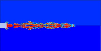
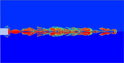
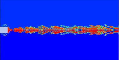
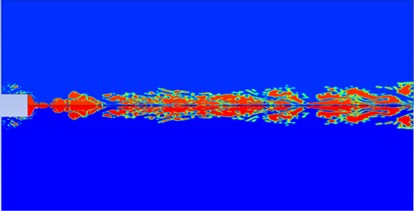
Fig. 1Contours of gas phase volume fractions at different instants
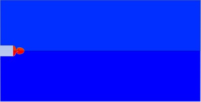
a) 1ms
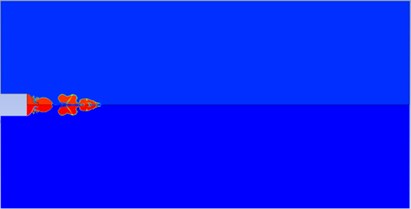
b) 12 ms
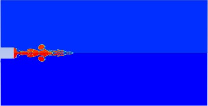
c) 17 ms
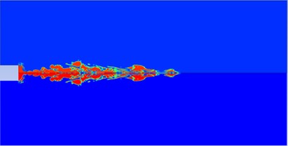
d) 47 ms
e) 73 ms
f) 94 ms
g) 135 ms
h) 194 ms
3. Wake noise analysis of underwater solid rocket motor
3.1. Computational model and boundary conditions
The expansion ratio of the nozzle was set to 1.63. The computational region is axisymmetric, the length is 114 times the throat diameter and the width is 34 times the throat diameter. The boundary conditions were set as follows: the entrance of the nozzle is the entrance of pressure, the total pressure is 9.8 MPa, the water free exit is set as the pressure exit, which is determined by the water pressure during the working phase of the nozzle. The water depth is set to 160 m, 260 m and 360 m, and the water temperature is set to 280 K by referring to relevant documents. The initial instant is set to the moment the pressure of the nozzle reaches the water pressure, which is 5 ms after engine ignition, and then the high temperature gas quickly fills the combustion chamber and nozzle. At this instant, the nozzle is filled with gas, the pressure is equal to the environmental pressure, and the temperature is 1120 K. Another 10 ms later, the pressure and temperature of the gas in the nozzle respectively increase to 9.8 MPa and 2800 K according to a linear law. The inner walls of the nozzle and the outer surface of the engine are treated as non-slip walls.
3.2. Growth process of gas bubbles in the wake field
The gas volume fraction contour is shown in Fig. 1. Through the simulation of the flow field, it can be concluded that the internal pressure of the nozzle is close to the pressure of the external water environment at the initial instant, namely the initial working moment of the engine. The gas pressure gradually increases due to propellant combustion. When the pressure value is greater than the maximum pressure value for the nozzle plugs, the plugs open, which promotes the formation of gas bubbles. The axial diffusion of the gas is slower than the radial diffusion due to the barrier of water, resulting in a trend of it rolling in all directions. Then, the gas bubbles start a process of “necking, expanding and necking” to continue their growth, and during this process both the pressure and velocity change. However, this process is not repeated indefinitely, the strength gradually weakens, resulting in a state of “dynamic balance” a few moments later.
3.3. Pressure and velocity distribution
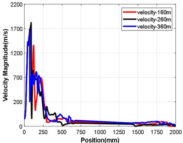
Figs. 2 and 3 show the nozzle velocity and pressure characteristics under different pressure conditions. It can be clearly seen from the pressure curve that the pressure fluctuations at the exit of the nozzle keep growing stronger and that the range in the fluctuations increases with an increase in water depth. At a depth of 360 m, the pressure variation is between 0.6 MPa-4.3 MPa, at a depth of 260 m, the pressure variation is between 0.38 MPa-3.2 MPa, and at a depth of 160 m, the pressure variation is between 0.36 MPa-2.4 MPa. It can be seen from the velocity curve that the velocity at the exit of the nozzle decreases with an increase in water depth, it is 1420 m/s at 160 m, 752 m/s at 260 m and 724 m/s at 360 m.
Fig. 2Axial pressure distribution at different depths
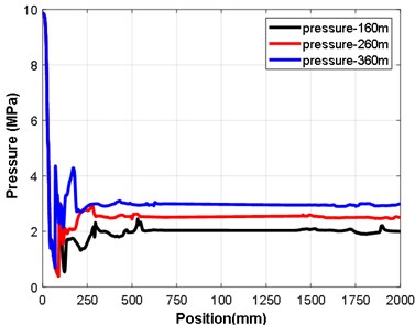
Fig. 3Axial velocity distribution at different depths
3.4. Noise analysis
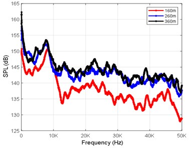
In order to obtain the noise characteristics of an underwater solid motor, 32 noise monitoring points in total are set for the computational simulation of three working conditions at depths of 160 m, 260 m and 360 m. The radial coordinates are [0 12 24 120 240 480 960 1200] mm, and the axial coordinates are [132 330 990 3960] mm. Figs. 4(a-d) show the sound pressure level curves of the monitoring points R17, R24, R25 and R32 at depths of 160 m, 260 m and 360 m.
Fig. 4Sound pressure level curve at each monitoring point
a) Sound pressure level curve of R17 (990, 0)
b) Sound pressure level curve of R24 (990, 1200)
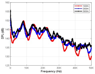
c) Sound pressure level curve of R25 (3960, 0)
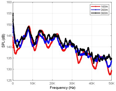
d) Sound pressure level curve of R32 (3960, 1200)
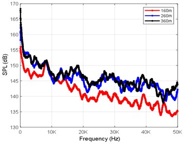
Spectrum analysis was conducted on the radiated noise results of the monitoring point R2 (132, 12), and the radiated noise spectrum is shown in Figs. 5(a-c). As can be seen in this figure, the radiated noise spectrum at different depths is characterized by a wide band and low frequency. At a depth of 160 m, the low-frequency components are mainly distributed in the range of 0-1.5 kHz and have an obvious peak value at 1 kHz. At the depth of 260 m, the low-frequency components are mainly distributed in the range of 0-0.6 kHz. For a water depth of 360 m, the low-frequency components are mainly distributed in the range of 0-0.4 kHz. According to theoretical analysis, it can be concluded that the nonlinear increase in the low frequency is mainly caused by an instability near the gas-liquid boundary in the jet flow. The peak sound pressure level of the noise source at the frequency of 1.0 kHz is mainly caused by the volume vibrations of the gas bubbles and the interactions between the bubbles under the action of the flow field force.
3.4.1. Axial attenuation characteristics
The attenuations along the axis and of each monitoring point on the axis were analysed, and the axial attenuation law at the frequency points of 1 kHz, 5 kHz, 50 kHz and 100 kHz was statistically analysed for a solid rocket engine at depths of 160 m, 260 m and 360 m. The analysis results are presented in Fig. 6(a-d) and Fig. 8(a-d). Fig. 6(a-d) show the axial attenuation characteristics of each frequency band at a depth of 160 m. Fig. 7(a-d) show the axial attenuation characteristics of each frequency band at a depth of 260 m. Fig. 8(a-d) show the axial attenuation characteristics of each frequency band at a depth of 360 m.
Fig. 5Spectrogram of R2
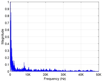
a) Spectrogram of R2 (160 m)
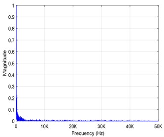
b) Spectrogram of R2 (260 m)
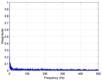
c) Spectrogram of R2 (360 m)
Fig. 6Variation law of axial attenuation at the depth of 160 m
a) Variation law of axial attenuation at 1 kHz
b) Variation law of axial attenuation at 5 kHz
c) Variation law of axial attenuation at 50 kHz
d) Variation law of axial attenuation at 100 kHz
Fig. 7Variation law of axial attenuation at the depth of 260 m
a) Variation law of axial attenuation at 1 kHz
b) Variation law of axial attenuation at 5 kHz
c) Variation law of axial attenuation at 50 kHz
d) Variation law of axial attenuation at 100 kHz
Fig. 8Variation law of axial attenuation at the depth of 360 m
a) Variation law of axial attenuation at 1 kHz
b) Variation law of axial attenuation at 5 kHz
c) Variation law of axial attenuation at 50 kHz
d) Variation law of axial attenuation at 100 kHz
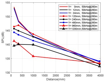
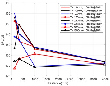
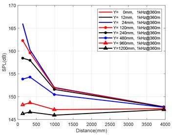
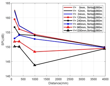
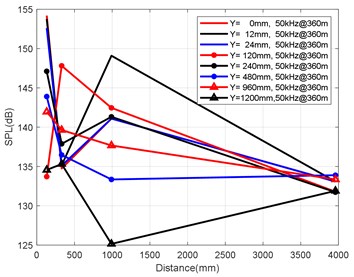
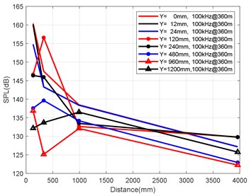
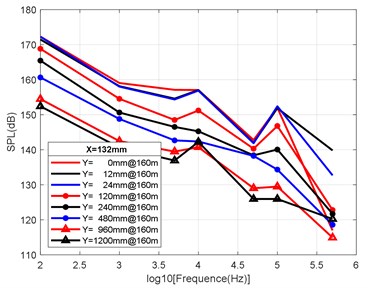
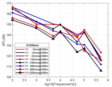
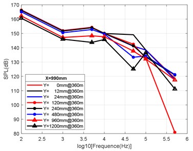
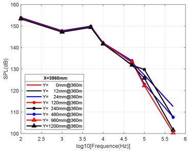
3.4.2. Attenuation of SPL with distance in the radial direction
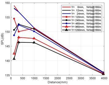
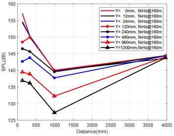
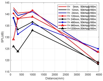
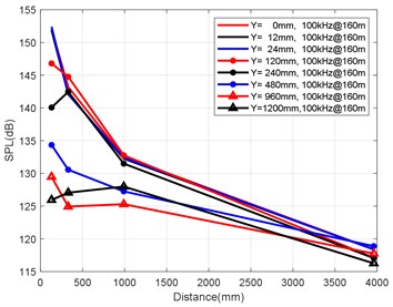
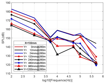
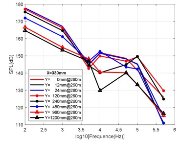
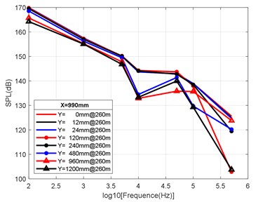
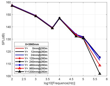
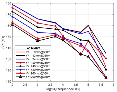
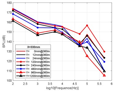
At the axial distance of 132 mm, 330 mm, 990 mm and 3960 mm from the nozzle mouth of the engine, the radial sizes of the monitoring points are 0 mm, 12 mm, 24 mm, 120 mm, 240 mm, 480 mm, 960 mm and 1200 mm, and the radial attenuation law was analysed. Fig. 9(a-d) show the radial surface attenuation characteristics of each frequency band at a depth of 160 m. Fig. 10(a-d) show the radial attenuation characteristics of each frequency band at a depth of 260 m. Fig. 11(a-d) show the radial attenuation characteristics of each frequency band at a depth of 360 m. The logarithm of the -coordinate is taken for the convenience of observing the radial attenuation law.
Fig. 9Variation law of radial attenuation at the depth of 160 m
a) Variation law of radial attenuation: 132 mm
b) Variation law of radial attenuation: 330 mm
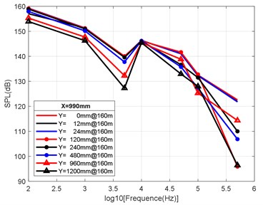
c) Variation law of radial attenuation: 990 mm
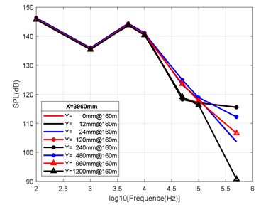
d) Variation law of radial attenuation: 3960 mm
According to the simulation results shown above and the axial and radial characteristics of the SPL measured at the monitoring points, the noise value is the total SPL at each frequency (the reference value is 10-6Pa). With an increase in axial distance, SPL gradually decreases, whereby the range becomes larger and larger, and the variation law remains almost constant with an increase in the distance. From Fig. 9(a-d) to Fig. 11(a-d), we can see that the SPL values are almost consistent between the radial sizes of 0 mm, 12 mm and 24 mm. In the axial direction of 132 mm at a water depth of 360 m, SPL is 174.02 dB, at 330 mm, the attenuation is 166.41 dB, at 990 mm, the attenuation is 160.59 dB, and for a distance of the nozzle mouth of 3960 mm, SPL becomes 153.94 dB. However, different monitoring points exhibit obvious increases or decreases in different frequency bands in different working environments. In the radial direction, SPL gradually decreases with an increase in distance, which is basically similar to the variation law in the axial direction. At 132 mm at a water depth environment of 360 m, the noise level is 174.02 dB in the radial direction of 100 Hz at 0 mm, the noise level is 174.01 dB at 12 mm, 173.99 dB at 24 mm, 173.27 dB at 120 mm, 171.73 dB at 240 mm, 168.34 dB at 480 mm, 163.16 dB at 960 mm, and 161.26 dB at 1200 mm.
It can be clearly seen that the closer the monitoring point is to the radial direction, the greater the noise level is, while the farther the monitoring point is away from the radial direction, the lower the noise level is. Moreover, at different frequency points of some monitoring points, SPL of the noise has similar values. For a stable engine, SPL decreases with an increase in frequency. At the same time, the SPL spectrum of each monitoring point is analysed, and the variation trend is found to be basically the same.
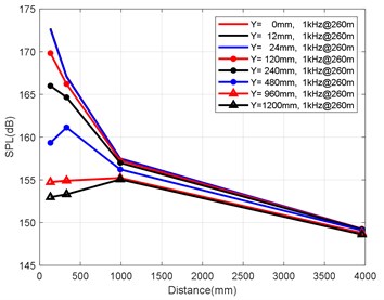
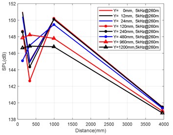
Fig. 10Variation law of radial attenuation at the depth of 260 m
a) Variation law of radial attenuation: 132 mm
b) Variation law of radial attenuation: 330 mm
c) Variation law of radial attenuation: 990 mm
d) Variation law of radial attenuation: 3960 mm
3.4.3. Experimental verification
In order to verify the accuracy of the numerical results, the noise pressure level of the engine wake field at 3 m depth was tested. Due to the confidentiality of the content of the experimental photos, the test results are shown in Table 1.
The numerical simulation method adopted in this paper is compared with the tank experiment (size of tank: 20 m × 7 m × 7 m) using a scaled model of an underwater high-pressure gas cylinder. The simulation and experimental results show that at a depth of 3 m, the SPL of the simulation is 3.2 dB-5.8 dB (3 kHz-5 kHz) higher than that of the experiment, and the SPL of the simulation is 2.4 dB-4.6 dB (5 kHz-10 kHz) higher than that of the experiment.
The results of both methods coincide well between 20 kHz and 50 kHz, with an error range of 1.1 dB-2.4 dB. It can be deduced that the numerical simulation method is applicable to the dynamic simulation of a flow field of the gas jet of underwater solid rocket engine, as well as for the simulation of the variation law of radiated noise.
Fig. 11Variation law of radial attenuation at the depth of 360 m
a) Variation law of radial attenuation: 132 mm
b) Variation law of radial attenuation: 330 mm
c) Variation law of radial attenuation: 990 mm
d) Variation law of radial attenuation: 3960 mm
Table 1SPL comparison between the experiment and the numerical simulation at a depth of 3 m
Monitoring locations (mm) | Method | SPL (dB) (3 kHz~5 kHz) | SPL (dB) (5 kHz~10 kHz) | SPL (dB) (20 kHz~50 kHz) |
(960, 0) | Tank experiment | 141.2 | 138.7 | 134.8 |
Simulation | 147.0 | 143.3 | 137.2 | |
(1200, 0) | Tank experiment | 128.7 | 123.4 | 115.0 |
Simulation | 131.9 | 125.8 | 116.1 |
4. Conclusions
1) The shape of the gas bubbles at the initial stages of the jet is regular at depths of 160 m, 260 m and 360 m. Because gas is constantly ejected, a tangential velocity difference exists at the gas-liquid interface, which leads to constant fluctuations in the gas-liquid interface and the processes of "necking-expansion-necking". This process is accompanied by constant variations in pressure and velocity in the nozzle and the gas bubbles. At the same time, there are obvious shock waves, i.e., the pressure undergoes periodic variations. After the stabilization of the jet, the pressure parameters at the axis of the nozzle remain unchanged with an increase in water depth, while the pressure at the exit of the nozzle fluctuates greatly. At a water depth of 360 m, the pressure amplitude reaches 4.3 MPa, and the velocities in both the axial and radial directions decrease.
2) The FW-H model is used to calculate the noise pressure of a supersonic gas jet of an underwater solid rocket engine. The research results show that the sound pressure in the wake field presents periodic pulsations, and that the peak value of the sound pressure decreases rapidly with an increase in distance from the receivers. This indicates that the sound wave weakens rapidly with an increase in distance, while the noise sound pressure level decreases with an increase in frequency. According to the spectrum analysis, the noise shows the characteristics of a wide frequency band and low frequency. The nonlinear increase in the low frequency is mainly caused by an instability near the gas-liquid interface under the jet flow, and the low frequency components are mainly distributed within a range of 1.5 kHz.
3) The numerical simulation method and an experiment with a scaled model at the depth of 3 m were used to compare the SPL at frequency bands of 3 kHz-5 kHz, 5 kHz-10 kHz and 20 kHz-50 kHz. The comparative results show that the numerical simulation method can be useful in research on the dynamic simulations of a flow field in the gas jet process of a solid rocket engine at a large water depth, as well as for the variation law of the radiated noise. Moreover, it also provides a reference for the design of underwater engines.
References
-
Zhang Youwei and Wang Xiaohong, “Numerical research on thrust peak for missile launching underwater,” Chinese Journal of Applied Mechanics, Vol. 24, No. 1, pp. 298–301, 2007.
-
E. O. Hoefele and J. K. Brimacombe, “Flow regimes in submerged gas injection,” Metallurgical Transactions B, Vol. 10, No. 4, pp. 631–648, Dec. 1979, https://doi.org/10.1007/bf02662566
-
C. W. Hirt and B. D. Nichols, “Volume of fluid (VOF) method for the dynamics of free boundaries,” Journal of Computational Physics, Vol. 39, No. 1, pp. 201–225, Jan. 1981, https://doi.org/10.1016/0021-9991(81)90145-5
-
Wang Cheng, Ye Quyuan, and He Yousheng, “Calculation of an exhausted gas cavity behind an underwater launched missile,” Chinese Journal of Applied Mechanics, Vol. 14, No. 3, pp. 1–7, 1997.
-
R. Scardovelli and S. Zaleski, “Direct numerical simulation of free-surface and interfacial flow,” (in Chinese), Annual Review of Fluid Mechanics, Vol. 31, pp. 567–603, 1999.
-
Y. L. Zhang, K. S. Yeo, B. C. Khoo, and W. K. Chong, “Simulation of three-dimensional bubbles using desingularized boundary integral method,” International Journal for Numerical Methods in Fluids, Vol. 31, No. 8, pp. 1311–1320, Dec. 1999, https://doi.org/10.1002/(sici)1097-0363(19991230)31:8<1311::aid-fld926>3.0.co;2-o
-
Zhong Fengquan and Lu Xiyun, “Numerical simulation of complex flow field for rocket launch under water,” (in Chinese), Journal of Astronautics, Vol. 21, No. 2, pp. 1–7, 2000.
-
Yi Shuqun et al., “Numerical simulation of the initial stage of noncondensing high-speed gas jet in liquid,” (in Chinese), Journal of Hydrodynamics, Vol. 17, No. 4, pp. 448–453, 2002.
-
He Xiaoyan, Ma Handong, and Ji Chuqun, “Numerical simulation of gas jets in water,” (in Chinese), Journal of Hydrodynamics, Vol. 17, No. 4, pp. 448–453, 2004.
-
A. V. Nguyen and G. M. Evans, “Computational fluid dynamics modelling of gas jets impinging onto liquid pools,” Applied Mathematical Modelling, Vol. 30, No. 11, pp. 1472–1484, Nov. 2006, https://doi.org/10.1016/j.apm.2006.03.015
-
A. Smolianski, “Finite-element/Level-set/Operator-splitting (FELSOS) approach for computing two-fluid unsteady flows with free moving interfaces,” International Journal for Numerical Methods in Fluids, Vol. 48, No. 3, pp. 231–269, May 2005, https://doi.org/10.1002/fld.823
-
S. Müller, P. Helluy, and J. Ballmann, “Numerical simulation of a single bubble by compressible two-phase fluids,” International Journal for Numerical Methods in Fluids, pp. n/a–n/a, 2009, https://doi.org/10.1002/fld.2033
-
Xiang Min et al., “Numerical simulation for underwater of solid motor tail flow,” (in Chinese), Journal of Propulsion Technology, Vol. 30, No. 4, pp. 479–483, 2009.
-
Zhang Shuai, “Research on character of solid rocket motor working deep underwater,” (in Chinese), Graduate School of National University of Defense Technology, 2012.
-
Zhang Shuai and Xiang Min, “numerical simulation of wake field of solid rocket motor working in deep water,” (in Chinese), in Conference Proceedings of Rocket Engine Professional Committee of Power Branch of Chinese Society of Aeronautics, 2012.
-
Jia Youjun et al., “Numerical simulation of underwater gas jet flow field,” (in Chinese), Solid Rocket Technology, Vol. 38, No. 5, pp. 660–663, 2015.
-
Wang Lili et al., “Numerical study of underwater supersonic gas jet for solid rocket engine,” Acta Armamentarii, Vol. 40, No. 6, pp. 1161–1170, 2019.
-
J. J. Gavigan, E. E. Watson, and W. F. King, “Noise generation by gas jets in a turbulent wake,” The Journal of the Acoustical Society of America, Vol. 56, No. 4, pp. 1094–1099, Oct. 1974, https://doi.org/10.1121/1.1903390
-
Zhang Wenping et al., “Experimental studies of submerged exhaust noise from diesel engine,” (in Chinese), Chinese internal Combustion Engine Engineering, Vol. 15, No. 2, pp. 52–56, 1994.
-
C. Tam, M. Golebiowski, and J. Seiner, “On the two components of turbulent mixing noise from supersonic jets,” in Aeroacoustics Conference, pp. 96–1716, May 1996, https://doi.org/10.2514/6.1996-1716
-
S. A. Stanley, S. Sarkar, and J. P. Mellado, “A study of the flow-field evolution and mixing in a planar turbulent jet using direct numerical simulation,” Journal of Fluid Mechanics, Vol. 450, No. 1, pp. 377–407, Jan. 2002, https://doi.org/10.1017/s0022112001006644
-
Ma Xianguo, “Emission behavior of acoustic noise of steam jet in subcooled water and experimental study,” (in Chinese), Journal of North China Electric Power University, Vol. 30, No. 1, pp. 35–40, 2003.
-
A. Niklas, E. Lars, and D. Lars, “A study of Mach 0.75 jets and their radiated sound using large eddy simulation,” in 10th AIAA CESA Aeroacoustics Conference Rome, pp. 1–24, 2004.
-
X. D. Li and J. H. Gao, “Prediction and understanding of three dimensional screech phenomenon from a circular nozzle,” in 13th AIAA CESA Aeroacoustics Conference Rome, pp. 1–19, 2007.
-
E. Groschel et al., “Towards noise reduction of coaxial jets,” in 13th AIAA CESA Aeroacoustics Conference Rome, pp. 1–18, 2007.
-
Wang Chunxu et al., “Experimental measurements of submerged free jet noise,” Journal of Ship Mechanics, Vol. 14, pp. 172–180, 2010.
-
Hao Zongrui et al., “Underwater noise characteristics of gas jet,” (in Chinese), Journal of Engineering Thermophysics, Vol. 31, No. 9, pp. 1492–1495, 2010.
-
Xing Junhua et al., “Numerical simulation and experimental validation of characteristics of jet noise from submerged axisymmetric nozzle,” Chinese Journal of Ship Research, Vol. 12, No. 6, pp. 49–53, 2017, https://doi.org/10.3969/j.issn.1673-3185.2017.06.008
About this article

