Sucker rod pump downhole dynamometer card determination based on a novel finite element method

1. Introduction

The average daily oil consumption has almost reached 100 million barrels per day in 2018 [1], having a share of about 34 % on global primary energy consumption. The proven reserves raised from 1696.6 billion barrels in 2018 [1] to 1729.7, whereas the average oil price for the type Brent dropped from 71.31 $ in 2018 to 64.26 $ in 2019, a tendency falling in early 2020. The statistical data indicate two significant points: total crude oil consumption will rise in the future, having a significant but slightly falling share within the next century. Proven oil reserves are climbing, and it is essential to mention that crude oil is irreplaceable today. Nothing can substitute its convenience in supply and energy density yet. Nevertheless, currently the oil price is going down or fluctuating because of economic instabilities.

Oil companies are pushed to reduce costs in all of their assets. In mature fields, where the wells are suffering under a high water cut, cost reduction is challenging. Still, it can be achieved by increasing the mean time between failures (MTBF) and energy-efficient operation of equipment. Sucker rod pumps are the preferred artificial lift system in low to moderate rate wells in these fields because of their high flexibility to adapt to changing reservoir conditions. Sucker rod pumps are used in so-called stripper wells that produce no more than 15 barrels a day. Many of these stripper wells have reached a depleted reservoir pressure state. This means that once they are shut in, they can never be economically restarted. Sucker rod pumps keep the majority of these wells alive. Improving pump efficiencies and the MTBF without adding considerably to operating costs, new technology can extend many of these wells’ economic life by years and raise the proven reserves by millions of barrels [2]. Fig. 1 presents the individual artificial lift systems’ market share as the percentage of wells equipped with a particular lifting technology. It can be seen that sucker rod pumps are installed in about 72 percent of all artificially lifted wells. This refers to about 600,000 units worldwide.

The principle of sucker rod pumping has been applied in the mid of the 19th century in the western hemisphere, first for oil production, even before the Chinese used this principle to lift water from the ground. However, this type of ALS is already applied for a long time, and the continuous improvement that has been introduced in the past, it is still indispensable to further advance sucker rod pump equipment on the one hand and the design methods, on the other hand, to keep it competitive and fit for the future.

Fig. 1Share of the significant artificial lift systems based on installed units [3]

Since the early days of sucker rod pumping, engineers and scientists are looking to predict and analyze the sucker rod pump. To mention an excerpt of work performed in the past acoustic signals of pumping systems have been used to detect the operation condition [4], the evaluation of equipment like plunger slippage models [5] and downhole desanders [6] has been performed in the laboratory and in the field. Extensive testing capacities have been constructed at the university to push the advances in sucker rod pumping [7], [8].

In this study, we introduce a novel Finite Element Method for the sucker rod pump downhole dynamometer card determination, present a comparison to a commercial software solution, the classical Gibbs’ approach, and real measured downhole cards.

2. Pump performance evaluation based on Gibbs’ approach

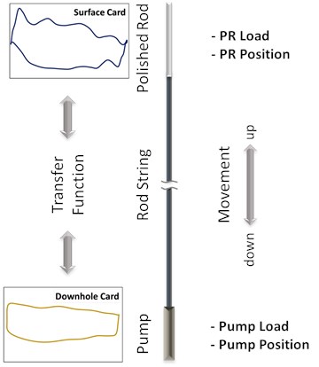
Fig. 2 gives an overview of the sucker rod pump analysis procedure. At the surface, the drive system generates the polished rod position. The drive system's speed is usually load-dependent, which results in a non-uniform movement of the polished rod. The polished rod movement is transferred to the downhole pump via the rod string, causing the pump's intake and discharge pressures, the load at the pump plunger. The plunger load interacts with the rod string movement and results in the polished rod load at the surface. Nowadays, sucker rod pumps are equipped with a load cell, which measures the polished rod load, and the walking beam position senor records the polished rod displacement.

Field engineers use two analytical procedures regularly – predictive and diagnostic analysis. The predictive analysis is used for designing a new and predicting the behavior of a not yet installed pumping system. The task is to select components and operating conditions, resulting in an optimized and efficient operation under the predefined boundary conditions. The challenges of this type of analysis are that no measured dynamometer data are available at the point of the design. The required input data to feed the model need to be approximated by mathematical models. The polished rod position and the pump plunger load need to be represented by estimations. Based on that, all other parameters can be evaluated. The diagnostic analysis is used to examine the behavior of already operating pumps. Polished rod load and position measurements are the boundary conditions for evaluating the plunger load and position. This information can interpret the working condition and any kind of malfunctions at the downhole pump.

Both approaches use a transfer function to describe the behavior of the sucker rod string. The sucker rod pumping system analysis’s quality is primarily based on this transfer function’s fundamental capabilities. In the field, sucker rod pumping systems operate under the most diverse conditions:

– The geometry of the wellbore: vertical w/o dog legs – inclined.

– Downhole pump setting depth: shallow – deep.

– Rod string: tapered rod strings, steel – fiberglass.

– Rod guides: number per rod, frictional behavior.

– Reservoir conditions: fluid composition, density, and viscosity.

Fig. 2Predictive and diagnostic analysis

The analysis of challenging pump installations requires a model that allows high flexibility, typically accompanied by a more complicated transfer function. In the past, several models with a different degree of complexity have been applied with multiple solution approaches. The following section summarizes the most important ones.

Gibbs [9] took the most significant step in describing the sucker rod string in the 1960ies. Many scientists have used his work as a basis for their research since then. He introduced the one-dimensional wave equation with viscous damping to describe a sucker rod string’s longitudinal vibrations in vertical wellbores as shown below:

In the above equation, $u$ is the displacement in the $x$-direction along the rod string, $t$ is the time; $a$ is the velocity of sound in the sucker rods, $x$ is the observed position, $v$ is a dimensionless viscous damping coefficient, and $L$ is the total length of the sucker rod string. Eq. (1) accounts for the stresses in the sucker rod string, inertia effects, and fluid friction in vertical wellbores. Gibbs [10] postulated that:

"…the viscous damping effect yields good solutions, even though non viscous effects such as Coulomb friction and hysteresis loss in the rod material are present. Fortunately, the non-viscous effects are relatively small, so the viscous damping approximation used in the wave equation is adequate…"

He solved this boundary value problem for a classical predictive analysis by defining the rod string's initial stresses, the polished rod's position, and the load at the downhole pump. The finite difference approach was used to solve the partial differential equation. Nevertheless, this approach can be used for diagnostic analysis too.

In 1967 Gibbs published the patent “Method of determining Sucker Rod Pump Performance” that introduced an analytical solution [9] for the diagnostic analysis using the viscously damped wave equation. The solution principle employed the separation of variables and product solutions. The boundary conditions were approximated with a truncated Fourier series. A sensitivity analysis of the significant model parameters found that ten to fifteen Fourier Coefficients are enough for most pumping situations to be analyzed. A surface dynamometer card consisting of at least 50 pairs of position and load values equally spaced in time is required for the best results when using the analytical solution. Sample data from 75 to 100 improve the accuracy of the calculation. The higher the dampening coefficient, the larger the area in the calculated surface card, and the more “rounded” it’s character. It seems that dampening factor $c=$$\pi av/2L$ in the range of 0.5 and 1.2 s^-1 gives good results in most applications. The maximum rod element length $x$ used should be between 150 and 230 meters. Finally, three pumping cycles are sufficient to eliminate the initial start-up effects [11].

Lekia and Day [12] introduced an alternative way to solve the viscously damped wave equation. This approach groups the fundamental variables affecting the operation of a total sucker rod pumping well system into eleven dimensionless numbers. The result consists of a set of design parameters for various pump size and depth production rate combinations where the optimum pumping mode can be selected.

In 2005 Hojjati and Lukasiewicz [13] presented a new technique for analyzing a sucker rod’s dynamic behavior, based on the Gibbs model, for a wellhead control system by the use of microprocessors. The main task was the simplification of the existing approach. In their paper, the problem is solved using D’Alembert’s equation system solution and an adaptive filter matrix method. The transfer matrix method has been proposed to model the rod's dynamic behavior of the sucker string. The technique's central concept is to replace the mathematical model’s solution with a simple matrix operation in which the pump force-displacement values are obtained as the product of the vector of the data at the polished rod and the transfer matrix. This is a fast mathematical operation, which can be performed hundreds of times during the period of a single stroke.

One of the latest developments was presented by Yang et al. [14]. In contrast to the existing solutions of viscous-damped-wave equation dynamics, they introduced a novel technique that allows a real-time estimation of the downhole situation. An infinite-differential state-space representation of the viscous-damped-wave equation dynamics was developed. Appropriate boundary transformations are applied. Spectral decomposition and truncation of an infinite number of modes were realized, and the viscously damped wave equation was cast into a system of coupled ordinary differential equations.

A significant step in developing an accurate model to describe the sucker rod string’s behavior in inclined wells was taken by Lukasiewicz [15] in the nineties. The presented model incorporates the curved sucker rod string’s dynamics, bending torques, and viscous and Coulomb friction, resulting from the rods’ contact with the tubing string. Based on a force balance in the direction of the rod string (Eq. (2)) and tangential to the rod string (Eq. (3)), a system of two differential equations was derived:

In the above equations $x$ represents the measured length along the curved rod, $\mu$ is the Coulomb friction coefficient, $S$ is the force in the curved rod's cross-section, and $\phi$ is the rod string’s inclination. $R$ is the actual radius of curvature of the curved rod, $A$ is the cross-section of the rod, $\rho$ the density of the rod material, and $\nu$ the fluid’s viscosity. The system of two partial differential equations was solved by the finite differences method. Lukasiewicz concluded that when applying a vertical well-designed model to analyze deviated wells' behavior, friction is mispredicted. The total friction would concentrate at the plunger, whereas, in reality, it is distributed along the rod in the inclined section. Finally, this fact would lead to further errors in the stresses and the rod string's calculations.

The principle of virtual displacement and differential geometry was used by Xu [16] to represent the deviated rod string dynamics by a set of six coupled differential equations. A numerical procedure based on the finite difference method and standard shooting technique is continued iteratively to converge to the steady-state solution with sufficient statistical accuracy. He reported that good agreement is shown between the computed results and field measurements.

In 2015 Araujo et al. [17] presented a model for deviated sucker rod strings without any path constraints. They suggested the well trajectory’s parametrization in three-dimensional space by the arc length and a vector description. Finally, the authors extended the numerical solution presented by Everitt and Jennings [18] to solve the model. In conclusion, it is recommended to investigate further the frictional behavior between rod guides and the tubing string and the tortuosity in specific sections, which can even be a problem in vertical wells.

The fast advancement in computer technology in the last decades allows the quick solution of large equation systems. The sucker rod string can be represented using spatial beam elements to derive the rod’s finite elements. The finite element method allows an analysis of the reciprocating motion of the sucker rod string and the occurring longitudinal vibrations, lateral vibrations, and torsional vibrations under various loads. Indicating the rod and tubing's contact friction state to obtain the rod vibration characteristics and the contact state with the tubing during the work process was presented by Jiang and Dong [19].

The latest advancement in the evaluation of pump cards was achieved by applying deep learning artificial neural networks. The analysis of the features of pump cards and identifying the sucker rod pumping system conditions is based on, e.g., Fourier descriptors. Neural networks can be trained to generate failure prediction models to recognize the rod pumping systems [20].

3. Dynamic finite element method analysis

The viscously damped wave equation is even used widely nowadays. Nevertheless, it comes along with some limitations. It is only valid for vertical wellbores, and the sucker rod string must consist of discrete uniform sucker rod elements, meaning that rod guides are not considered in the analysis. Hence, the rod guides – tubing contact behavior and the friction between sucker rods and tubing in inclined sections are not accounted for.

Advanced finite element method (FEM) analysis is used in various applications in various industry sectors and provides a very accurate way to analyze complex processes, like the sucker rod string [19]. This publication builds on the knowledge of existing FEM analysis and presents a novel dynamic finite element method to evaluate the sucker rod pump downhole equipment's performance. Downhole pump and rod string parameters can be determined for standard and new advanced designs, like the SRABS Sucker Rod Anti-Buckling System [21], [22], [23], [24].

3.2. Model of the sucker rod pumping system

The finite element model of a sucker rod pumping system needs to account for the equipment installed in a real well. The tubing and the sucker rod string with the molded rod guides, all located concentrically along the borehole axis, have to be represented and modeled. A wellbore model using Abaqus 2020 is created in the so-called input file, which provides the finite elements solver with the relevant model data and information. Defining an input file includes the following steps [27]:

– Creation of nodes and node sets, representing the wellbore geometry.

– Creation of elements, element sets, assignment of material properties, representing installed equipment.

– Definition of contact behavior.

– Definition of boundary conditions and time-dependent amplitudes, representing load and displacement.

– Definition of the simulation steps.

3.2.1. Nodes and node sets

The coordinates of the borehole’s trajectory are the basis for the model generation. The entire trajectory’s implementation is one of the key points of this approach and significantly increases the analysis's accuracy. Wellbore coordinates taken from the borehole survey are interpolated by cubic spines between the measurement points and processed into the model's required nodes. Nodes for the same equipment type, e.g., nodes along one section of the rod string, are combined into node sets. The cubic spline coordinates of the wellbore axis are used to model the rod and tubing string.

3.2.2. Elements and element sets

The sucker rod string is represented by three-dimensional, quadratic beam-elements, so-called B32 elements [28]. The elements consist of three nodes, each with quadratic interpolation functions. Elements for the same rod string section are combined to one element set and assigned with a cross-section. The rod string installed in the wellbore is not just a straight rod, but auxiliary equipment, like rod couplings and rod guides, is attached. A non-structural weight is defined to account for the component’s weight.

Material properties such as density $\rho$, Young’s modulus $E$, and Poisson’s ratio ν are assigned to the elements. Linear elastic material behavior is defined [29]. Since the sucker rod string is made of steel, the density, Young’s Modulus, and Poisson’s Ratio assigned to the elements are 7850 kg/m³, 210 GPa, and 0.3, respectively. The tubing is modeled by using the same coordinates as the rod string. As tube-to-tube contact elements represent the tubing string, separate tubing elements are not required.

3.2.3. Contact definition

Contact behavior is modeled by applying the tube-to-tube contact elements, which account for the finite-sliding interaction between two pipes where one pipe is located inside the other – the outer pipe represents the tubing the inner represents the rod string. These particular elements assume that the two strings’ relative motion is taking place mainly along the line, defined by the rod string axis [28]. The implementation of tube-to-tube contact elements consists of three distinct steps: the definition of the contact elements and contact element sets, the interface generation, and the slide line definition.

The contact elements are defined based on the rod string’s single node set and combined into the contact element set connected to the slide line. Contact has to be established between rod guides – tubing and between sucker rods – tubing. Based on the different contact surfaces, each rod string section contains two contact element sets. The ITT31 tube-to-tube contact element type is selected, an element in 3D space with linear interpolation functions.

The element’s interface is used to assign element section properties to the contact elements. The essential property, referring to contact, is the radial clearance between the contact surfaces. The radial clearance is the distance between the tubing's inner diameter and the contact partner, rod guides, or rod string. The radial clearance between the rod guides and tubing's inner surface is defined based on measurements with one millimeter. The rod string section's diameter defines the radial clearance between the tubing's inner surface and the rod string under consideration.

The slide line’s definition is the connection between the tube-to-tube contact elements and the slide line’s nodes. Here the center of the tubing string is defined as the slide line. The slide line definition comes along with the friction coefficient between the contact pairs. The friction coefficient for the contact tubing – rod guides is defined with 0.1 and for tubing – rod string with 0.15 [30].

3.2.4. Boundary conditions and load / displacement amplitudes

One needs to distinguish between the boundary conditions of the tubing and rod string. The tubing is assumed to be fixed through the tubing hanger at the wellhead and a tubing anchor in the well. Hence the tubing is static; no tubing displacements or rotations are allowed during the entire simulation. It is accomplished by constraining all 6 degrees of freedom of the tubing’s node-set.

When focusing on the uppermost node’s motion (UN), the polished rod, and its boundary conditions, it needs to be taken into account that the rod is reciprocating along the wellbore axis only, and no rotation takes place. This is ensured by constraining the corresponding degrees of freedom of the UN.

The displacement of the polished rod is applied by prescribing a displacement boundary condition. It states that the UN is subjected to a displacement in the vertical direction at the stuffing box given by an amplitude parameter that directly accesses the pump stroke data measured by the dynamometer. The load amplitude refers to the load measured at the polished rod. At the bottom node, which refers to the node at the end of the rod string, where the downhole pump is connected, a dynamic concentrated plunger load of unknown magnitude is applied. The direction of this load remains constant during the entire pump cycle. It is defined by the unit direction vector of the tangent passing through the lowermost point of the rod string.

3.2.5. Simulation steps

The first step in the simulation is to apply gravity to the system. Gravity does not influence the fixed tubing string. The movement of the rod string, subjected to gravity, is fully constrained at the UN. The rod string is hanging in the wellbore while being fixed at the polished rod and kept in place by the tubing string. This step is maintained for the first series of time increments. To prevent excessive oscillations of the rod, the gravity load is ramped up to its full magnitude. As soon as the first step is completed, the polished rod’s displacement is applied at the UN. At the bottom node, the plunger load approximation is applied.

The keyword moderate dissipation is added to the dynamic step definition. This purely numerical parameter will choose a method with larger than default numerical damping and a more aggressive time incrementation scheme at some acceptable expense of solution accuracy.

3.2.6. Downhole information retrieval

This paper aims to show an advanced numerical solution for determining the performance of the downhole pump. A very efficient way to perform this task is applying an iterative procedure. The nature of FEM does not allow the direct evaluation of the plunger load, based on polished rod load and position. The plunger load is determined for incremental time steps by a unique search algorithm, controlled by an automated script. Experience has shown that the time increment can remain constant for the entire pump cycle. Fig. 3 shows the iterative procedure.

In the beginning, an initial plunger load value is selected for time step zero. After completing the first simulation run, the vertical reaction force at the uppermost node (polished rod) can be evaluated and compared to the measured one. A divergence beyond the user-defined tolerance causes an adjustment of the initial plunger load and a repetition of the simulation for this time step. Depending on the divergence sign, the applied plunger load is increased or decreased by a defined magnitude. As long as the user-defined tolerance is not reached, the procedure is repeated. If the simulated plunger load value is, based on the UN load value, accepted, the procedure continues with the next time increment. This iterative procedure is conducted for every time increment until the full pump cycle is completed and the entire evolution of the plunger load has been obtained until the simulation time reaches the stroke duration.

Fig. 3Iterative procedure [29]

A convenient way of implementing this approach in a FEM solver is by creating restart files for each time increment. A restart file is built on the master input file, containing all relevant model data, but the user can adjust properties. In the presented application, the quantities, which differ from restart file to restart file, are the polished rod position and the selected plunger load.

4. Pump card reference data

The performance of this novel simulation method is demonstrated on a vertical and deviated sucker rod pumping system. The sucker rod pump, installed in the deviated wellbore, is equipped with a standard downhole pump. In contrast, the sucker rod pump in the vertical wellbore drives the Sucker Rod Anti-buckling System (SRABS), a novel downhole pump.

4.1. Deviated well – standard SRP only

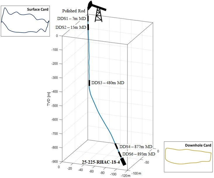
The system, being simulated, is situated in a mature oil field and operated under pump-off conditions. The downhole pump is a 25-225-TH-18-4, referring to a 2.25 in tubing type pump size installed as part of a 2 7/8 in tubing string. The tubing string is anchored in a true vertical depth (TVD) of 884 m, respectively, in a measured depth (MD) of 906 m as shown in Fig. 4. During the observed duration, the well produced about 8.8 m³ of fluid per day at a water cut of 85 %, and a solution gas ratio of 23 sm³/sm³. No significant problems with paraffin or fines have been reported. At the observed time, the well was equipped with 7/8 in sucker rods, no sinker bars, and four pieces of rod guides per rod segment. The reservoir layer this well produces from is located at a depth of about 955 m TVD. At the downhole pump’s setting depth of 900 m, the wellbore reaches an inclination of about 30 degrees. The kick-off point of the well is located at a depth of 480 m. Borehole logs have indicated a maximum dogleg severity of 3 deg/30 m. At the surface, a conventional pump jack with the designation C-320D-256-144 is driven by a motor with variable speed drive control and operated at three strokes per minute.

Fig. 4Trajectory of the deviated well

Measured downhole rod string data are available for the chosen deviated system. Five downhole dynamometer sensors (DDS) were installed along the rod string (see Fig. 4). Two DDS were installed next to the polished rod, one at the well's kick-off point and two DDS next to the pump plunger [31]. Each DDS recorded the stress state, the three-dimensional movement, and the installed position's surrounding temperature. The verification of the device recordings was done by comparing the polished rod load with DDS1 and DDS2.

The downhole dynamometer sensors have been installed as part of a well workover. As part of this operation, the wellbore was flooded with workover fluid. After the pump’s restart, removing the workover fluid is indicated by a full pump card and low fluid load. Fig. 5 presents the loading for DDS 1 and DDS 6. It indicates a change in the pump conditions after about 80 hours after the restart. The fluid in the annulus was lifted entirely, and due to the poor reservoir performance, the pump condition switched to pump off. The degree of this pump-off situation increases with time until stabilization has been seen after 180 hours of pump operation. The pump condition change came along with an increase in fluid load, as the fluid level and the intake pressure dropped until the pump depth was reached.

Fig. 5DC measurements – deviated well [31]

The chosen point in time, used as the basis for applying the novel finite element method, was recorded after 180 hours of pump restart. This point was selected as the pump card trend indicated the first static balance between reservoir performance and pump rate. Fig. 6 presents the surface dynamometer card and the pump card at this point.

Fig. 6DC measurements, 180 hours after pump restart – deviated well

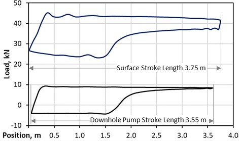
The surface card indicates a stroke length of 3.75 m, a peak polished rod load of about 45 kN, and a minimum polished rod load of 23 kN. Low rod string dynamics are the result of the low number of strokes. Severe pump-off can be seen as well. The measured pump card indicates a reduction in stroke length to about 3.55 m. A maximum load of 9,5 kN and a minimum load of –4 kN is shown.

4.2. Vertical well – standard SRP and SRABS

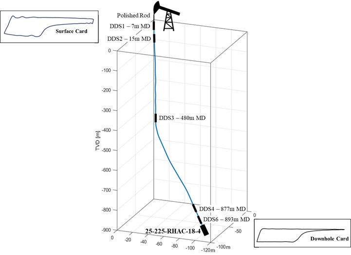
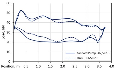
This sucker rod pumping system is installed in a vertical well situated in the same basin as the deviated system. This system is part of a large research project, and intensive monitoring takes place since 2017. The wellbore is equipped with an 800 meter long anchored 3 1/2 inch tubing string. From the beginning of the research project until mid of June 2018, the system was equipped with a standard 30-225-RHAC-18-4 downhole pump. The pump was set at 800 m and operated at 8.57 strokes per minute. The rod string comprises 280 m of 1 inch rods grade D, 490 m of 7/8 inch rods grade $D$, and 30 m of 2 inch sinker bars. The recorded fluid properties were 25° API oil gravity, a 113 Pa/m gas gravity, and 98.8 % water cut. The dynamic fluid level was measured to be at 475 m from the surface, a casing head pressure of 11 bar, and a tubing head pressure of 8 bar were seen. The standard pump's gross production rate was 90 m³/day. A variable speed drive drives the C-320D-256-144 pump jack. Fig. 7 shows the dynamometer card, taken mid of February 2018. The peak polished rod load is 52 kN, the minimum polished rod load is 20 kN, and the stroke length is 3.74 meters.

In June 2018, the standard sucker rod pump was replaced by the sucker rod anti-buckling system (SRABS). SRABS is a new system that reduces the compression in the rod string during the downstroke and effectively prevents buckling without using sinker bars and similar equipment [24]. The SRABS pump is installed with a similar rod string as the standard pump to enable a simple comparison of the downhole pump performance. The operation conditions are kept equal.

Fig. 7 indicates similar stroke peaks and minimum polished rod loads. Nevertheless, the card area, which represents the energy consumption, is smaller for SRABS.

Fig. 7Standard pump vs. SRABS - vertical well

5. Gibbs’ solutions

The presented analytical solution is based on Gibbs [9]. This method is used because of its simplicity and popularity in evaluating the downhole performance for vertical and even inclined sucker rod pumping systems. The start point for this analytical solution is the preparation of the load boundary condition, which is calculated by subtracting the rod string weight from the surface dynamometer card. The subsequent step is decomposing the load boundary by the Fourier series and the pump card calculation. For the presented analysis, 20 Fourier coefficients have been chosen, as this number adequately represents the load boundary condition. The commercial software product is a standard tool used in the industry. For comparison reasons, the vertical package is applied.

5.1. Deviated well

Fig. 8 presents the results of the analytical solution, including a sensitivity study of the damping coefficient. This damping coefficient is the only unknown when using the Gibbs’ approach. When taking a closer look it can be seen that the calculated results do not accurately fit the measurement data. The reason is simple – the Gibbs’ approach is derived for vertical wells only, but the wellbore under investigation has a significant inclination at the pump’s setting depth.

Fig. 8Gibbs’ solutions compared – deviated well

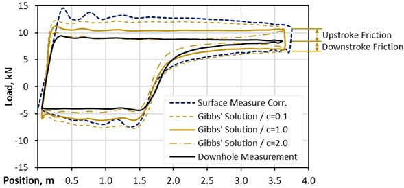
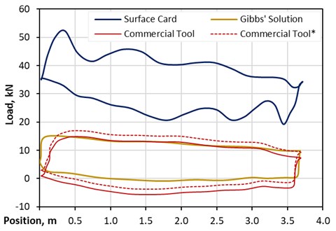
The rod string friction is falsely interpreted as plunger friction [15], as shown in Fig. 8. A reasonable magnitude of the damping coefficient c prevents, on the one hand, a severe oscillation of the plunger load, which would be the situation if the magnitude of c is minimal. On the other hand, too large magnitudes of c would cause reverse ballooning of the pump card. For the selected example, c equal to one seems to show a good fit. Nevertheless, Gibbs indicates that Coulomb friction effects can be simulated by choosing appropriate damping coefficients [10]. According to Fig. 8, a damping coefficient of two would reconstruct the measured pump card, except at the end of the upstroke. Fig. 9 shows the comparison of the measured pump card, the analytical solution with c equal to one, and the result from the commercial product. It can be seen that the analytical method can be used to correctly predict the behavior of the pump, even for inclined well, with a workaround.

Fig. 9Overall comparison - deviated well

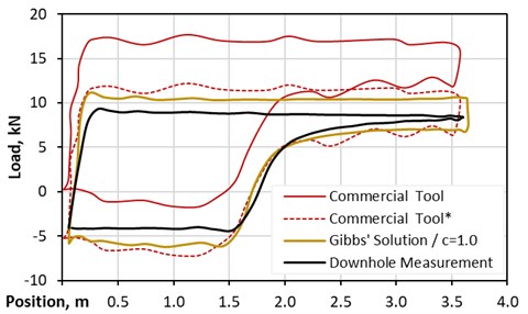
The commercial product results showed that the pump card’s width at the end of the upstroke is comparable with the results of the analytical solution and represents the coulomb friction in the inclined section. Nevertheless, the line denoted as Commercial Tool* shows that the whole card’s offset is about 5500 N.

5.2. Vertical well

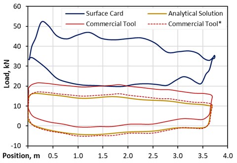
Both pump types have been analyzed with the analytical method and commercial product. Fig. 10 presents the results of the standard pump evaluation. The blue line represents the surface card, the brown line the analytical solution’s solution, and the full red line represents the commercial software results. It can be seen that the shapes of both solutions fit very well; just the offset is incorrect. A closer investigation of the forces acting on the rod string during the downstroke, which are pressure force and friction, results in a compressive load of about 3500 N. The Gibb’s approach showed a good match, whereas, the commercial product’s solution needs to be shifted by 4500 N downwards, denoted as Commercial Tool*.

Fig. 10Pump card comparison – vertical well standard pump

Different results have been seen for the evaluation of the SRABS pump. The construction of this type of pump reduces a significant portion of compressive load during the downstroke. Evaluations resulted in a compressive load of about 500°N during the downstroke for the vertical well configuration. The Gibb’s approach can predict the SRABS pump behavior and confirms the low compressive load (Fig. 11). In comparison, the offset and the shape of the pump card are incorrectly predicted by the commercial product. Even an offset shift of about 2000 N does not show a satisfying fit. This finding is based on the fact that the commercial product is not built to analyse customization pumping systems.

Fig. 11Pump card comparison – vertical well SRABS pump

Additional information, like rod guide – tubing contact forces and buckling effects, are of big value for the redesign and system optimization. The Gibbs’ approach cannot provide that information. The shown analysis has demonstrated the need for advanced, precise predictive software to handle the performance prediction of standard and novel pumping systems.

6. FEM solutions

The presented advanced FEM simulation to determine the downhole pump card is applied to both, the deviated and the vertical wells. The applied FEM simulation is capable of providing all the requested information about the dynamics of the rod string – tubing interaction [32]. The simulation is performed with constant time increments of 300 milliseconds, which has shown an appropriate balance between the accuracy of the results and the computational costs. The simulation run acceptance criterion for the polished rod load was set to 1000 N. This means that the difference between the reaction force evaluated at the UN of the FEM simulation and the measured dynamometer load needs to be smaller than 1000 N to move forward to the next step. The reduction of this acceptance criterion to a smaller value increases the computation duration disproportional to the improvement of the resulting quality.

6.1. Deviated well

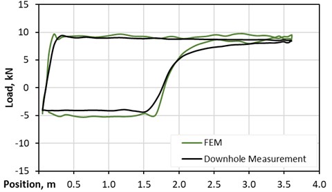
The deviated system results are compared to the DDS measurements. One of the specific features of this advanced FEM approach is the full implementation of the wellbore trajectory, which significantly improves the resulting quality. Fig. 12 shows an exact match of measurement and simulation results.

Fig. 12FEM solution compared – deviated well DDS6 120 h

6.2. Vertical well

No downhole measurements are currently existing for the vertical system. As a result, the FEM solution is compared to the analytical solution. Fig. 13 compares the FEM and the analytical solution for the vertical wellbore and the standard pump. It can be seen that the agreement between the FEM solution, represented by the grey line, and the analytical approach, displayed by the brown line, is very good. The main difference between them is identified at the beginning of the upstroke, where the analytical approach does not capture the fluctuating tensile stresses downhole as a result of the fluid inertia effects, representing the peak plunger load.

Fig. 13FEM solution compared – vertical well standard pump

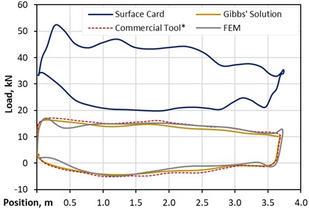
Fig. 14 compares the FEM and the analytical solution for the vertical wellbore and the SRABS pump. Also, for this new, innovative downhole pump, the FEM solution has a good agreement with the analytical solution. Compared to the standard pump’s downhole card, the oscillations during the upstroke, which are part of the FEM solution, are slightly increased.

Fig. 14FEM solution compared – vertical well SRABS pump

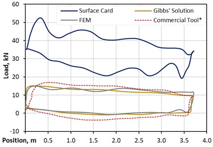
Remarkably, the plunger load during the downstroke is just slightly negative and close to zero, meaning that almost no compressive loads are present. The commercial product in this case is located closer to both the FEM solution and the analytical approach as compared to the previous case, nevertheless an offset correction was applied.

The simulation results confirm the working principle of SRABS. The significance of these results cannot be overemphasized, as they show in detail that the SRABS system can impact the dynamic behavior of the sucker rod string in such a way, that only tensile stresses prevail. This in turn means that buckling of the rod string can be prevented and the lifetime of downhole components is extended.

By applying the novel FEM method for downhole pump card evaluation, the most accurate solution is obtained as a complete description of a sucker rod pumping system is implemented. This means that the full trajectory of the corresponding wellbore is taken into account, whereas the friction between the rod guides and the tubing and also between the rod string and the tubing is included as well. The considerable advantage of understanding the sucker rod string’s downhole dynamic behavior is that highly accurate statements in terms of fatigue modeling can be made, as the buckling behavior of the string can be predicted. The approach of predictive maintenance concerning the rod string can also be lifted to the next level, meaning that proper estimates of when to replace downhole equipment can be made. Hence, this innovative FEM diagnostic tool aids in decreasing the number of buckling-induced failure incidents in sucker rod pumping. From the economic point of view, the mean time between failures will be increased and therefore the economic limit of a well will be postponed.

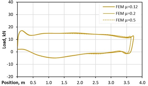
6.3. Impact of friction coefficient

The advanced finite element method approach is working with physical parameters, like material properties or friction parameters. Mainly, friction coefficients are depending on the conditions of the investigated wellbore. This section shows a sensitivity analysis of the friction coefficient for the tubing – rod guide contact. The standard value for the friction coefficient between the rod guide and tubing used in the FEM simulations is 0.1. To determine its actual impact on the downhole card performance, the simulations are evaluated for friction coefficients of 0.2 and 0.5, while all other parameters remain unchanged. A graphical representation of the results is shown in Fig. 15. The obtained values for the plunger load values of the individual simulation runs are almost identical, which means that the impact of the friction in the case of vertical borehole trajectories is negligibly small.

Fig. 15Impact of friction coefficient – vertical well standard pump

7. Conclusions

Nowadays, the majority of artificially lifted wellbores are operated by Sucker Rod Pumping units. Hence, a safe, economical, and efficient operation of this lifting method must be guaranteed. Over the last decades, numerous techniques to determine the sucker rod pump performance have been used with limitations. Typically, most models require somehow arbitrary parameters to define the damping of the system.

The presented novel advanced finite element method overcomes this limitation and only uses physical parameters. Besides, the full 3D trajectory can be implemented, while at the same time, the friction between the string and the tubing as well as friction between rod guides and tubing are considered. The innovative iteration algorithm, implemented by a powerful automated script, manipulates the input file and the FEM solver. The reaction force at the simulation's surface shows remarkable agreement with the measured surface dynamometer card. Moreover, the numerically obtained plunger load corresponds to the measured plunger load, proving the validity of the shown calculation model.

The model predicts rod string behavior and is applied to reduce the amount of rod string failures caused by buckling or fatigue, which substantially increases the mean time between sucker rod pumping units’ failures. The effective use of this advanced finite element method allows a significant reduction of costly interventions, which is closely linked to lost time incidents. It will postpone the economic limit of a well and also increase the recovery factor. The presented method is a very flexible approach and can simulate standard sucker rod pumping systems and novel designs.