Sucker rod pump frequency-elastic drive mode development – from the numerical model to the field test

1. Introduction

The artificial lift market will experience substantial growth in the forthcoming decade, where sucker rod pumps will take a significant share [1]. Sucker rod pumping systems represent the oldest and most widely used artificial lift method with several hundreds of thousands of units worldwide [2]. Their application ranges from lifting oil in mature conventional oil fields, production in stripper wells and unconventional oil fields, to unloading gas wells. Stripper wells represent a high percentage of vertical oil wells and produce less than 10 barrels per day. Sucker rod pumps (SRP) are well known for their flexibility to match the well capacity during the natural decline in production; they can be used to maximize the drawdown in the well, have high efficiency, and a relatively simple design. The system can lift high-temperature and viscous oils. Scale and corrosion treatments can be performed efficiently during the operation [3].

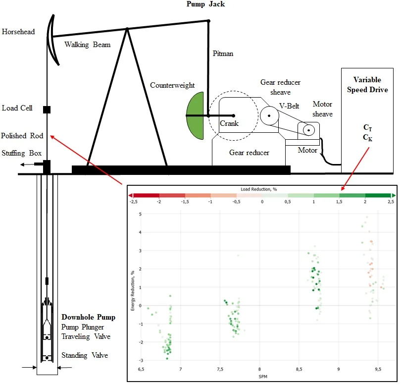
The sucker rod pumping system is composed of the surface unit, the sucker rod string, and the downhole pump. The surface unit, called the pump jack, represents the drive of the system. Fig. 1 presents the schematics of the conventional pump jack design.

Fig. 1Sucker rod pumping system

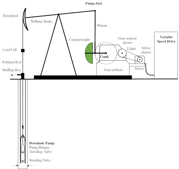
The first section of the pump jack reduces the rotation speed, whereas the second transforms the rotation into translation. The electrical motor’s sheave drives the V-belt, which drives the gear reducer sheave and represents the first stage of speed reduction. The gear reducer sheave is positioned at the two-stage gear reducer input shaft, which further reduces the rotation speed. At the output gearbox shaft, the final speed is obtained. This transmission system typically reduces a motor speed of 1,000 rpm by a factor of about 150 to 200. Finally, a system speed in the range between 3 and 15 rpm is reached. The cranks carry the counterweight, which balances the rod string's weight and is connected with the pitman. The pitman is connected to one end of the walking beam. On the other end of the walking beam, the horsehead is positioned. The horsehead’s wireline hangers carry the polished rod, which passes through the wellhead’s stuffing box. The polished rod is connected to the sucker rod string, which transmits the pump jack’s motion to the downhole pump plunger.

During the upstroke of the downhole pump’s plunger, the traveling valve as part of the plunger is closed, the fluid load is carried by the rod string and lifted. Simultaneously, the standing valve is opened to allow inflow into the pump’s intake chamber as part of the fixed barrel. During the plunger’s downstroke, the standing valve, which carries the fluid load now, is closed, and the plunger moves through the fluid column back to its bottom dead center. The cyclic load changes cause dynamics in the pumping system, which need to be handled by the pump jack [4]. Continuous research on the optimization and improvement of surface and downhole components [5], [6], [7] of the pumping system is performed in the laboratory [8], [9] and the field.

The electric motor can be driven directly from the electric grid or by a frequency converter. The electric grid's direct connection is a cheap solution but requires additional hardware, a so-called soft start, and a change in the belt pulley sizes to adjust the pump’s strokes per minute. Using frequency converters (FC) for industrial pump applications is state-of-the-art and provides many advantages, like controlling the speed of rotation and torque of the equipment and reducing the grid load at start-ups through limiting the inrush current. Many publications deal with FC and electric motor combinations for specific applications, increasing efficiency or power density, enhancing control strategies, or extending the power capacity [10]. A sucker rod pumping system driven by a frequency converter is known as a variable speed drive system (VSD). Conventional VSD applications change the motor speed independent of the supply grid frequency. A high degree of flexibility is achieved to adjust the pump speed to the reservoir’s performance. Nevertheless, after a smooth start-up, typically, a constant motor frequency is chosen. More recent FC generations enable bi-directional power flow, which refers to a so-called active front-end. Otherwise, the regenerative energy of the system would be burned at the DC-link brake resistor, resulting in an efficiency reduction. One major drawback of the VSD technology is the higher acquisition costs. It is also common for higher power ratings that several FC share one input stage and DC-link. The energy can then be balanced between the connected electric motors.

Studies of SRP electric drives have shown a low motor efficiency for regular and conventional VSD systems. The reason is seen in the load oscillations of polished rod and counterweights. These load fluctuations change the power factor's characteristics, which vary within a wide range and drop the performance. Accurate counterbalancing is recommended to improve motor efficiency [11]. In the past, low efficient ultra-high slip motors have been used at the expense of efficiency to improve the system's elasticity and reduce peak loads and power requirements. Khakimyanov and Khusainov [12] showed how to utilize counterbalancing weight to increase efficiency and reduce oil production costs. Solodkiy et al. [13] discussed a sensorless method of a pumping unit and optimal counterbalancing methods within the control algorithm for nonlinear pumping loads. The capabilities of a FC are far beyond enabling just variable motor frequency. Several publications have presented different approaches to change the motor speed within one cycle to improve the SRP system.

Pumping units' variable-speed drive technology is seen as one of the most advanced energy-saving technologies applied in oilfields. FCs overcome the pump jack’s limitation of the four-bar mechanism to achieve a full-cycle variable speed-controlled operation. Ferrigno et al. [14] studied the downhole plunger speed in high gas-oil ratio and high friction wells. The plunger speed calculation, based on the viscous damped wave equation algorithms, enabled a comparison with other external tools that consider Coulomb friction and its effects in deviated wells. The operation mode of the frequency converter was adjusted to prevent regeneration by accelerating the motor. Successes have been seen in a field test with 50 pumping systems. A flexible variable frequency driving system was designed for reducing energy consumption in a low rate oil field in China to control pumping speed in real-time [15]. With SPM below one stroke per minute, the super-slow systems' optimization has shown a system efficiency improvement from 11.8 % to 18.02 %. The automated and closed-loop control algorithm reduced the operator’s demand to monitor the day-to-day production. A model, accounting for the system dynamics and the beam pumping unit under variable speed driving conditions, has been shown by Chaodong et al. [16]. Their optimization criterion is the reduction of power consumption. The model’s application on ten wells has shown a significant power saving rate, gear reducer peak torque reduction, and a system efficiency increase. However, Zi-Ming et al. [17] concluded that fully coupled dynamic models, accounting for the motor, pump jack, rod string, and downhole pump, still need more investigations. Several issues that might be caused by the entire variable speed operation, like the energy-saving mechanism, the influence of inertial load caused by moving parts, and counterbalance adjustment, still need to be investigated. Palka and Czyz [18] have demonstrated that the sucker rod pump efficiency can be improved significantly by implementing a defined variable speed of the prime mover. Based on a Fourier series representation of the motor speed, a search algorithm was defined to look for the Fourier coefficients, which maximize production while satisfying the system constraints, like motor torque and speed, stresses in the rod, and energy consumption to determine the optimum motor-speed profile. Field tests showed an increase in production without increasing energy consumption or loads in the system of up to 133 %. New developments of downhole equipment [19], [20], [21] and surface operating procedures can help to improve CO₂ lifecycle footprint of the oil production by sucker rod pumps.

This publication presents a fully coupled dynamic model of the downhole and surface components, used to evaluate the novel frequency elastic drive mode approach for sucker rod pumping systems. The field tests show the verification of the model and its capabilities. Compared to many others, the proposed method, introduced in this publication, does not require hardware adjustments or affect the controller code or parameters itself; just the reference value calculation of the speed controller is modified. In addition, the capabilities of the wire rope technology, which represents an alternative to the standard rod string are shown.

2. Methodology: frequency-elastic drive mode

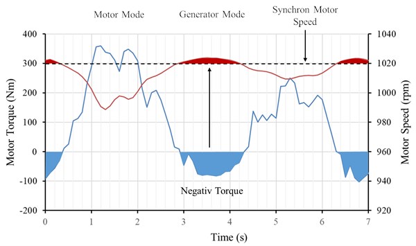
The motor speed and torque evaluation have shown that a conventionally driven sucker rod pump is a very rigid system. A large torque is required during the polished rod’s upstroke and the upwards movement of the counterweights. Fig. 2 indicates that a negative torque is generated by the system, which causes the motor speed to pass its synchronal speed and change the motor’s operation mode into a generator. The energy generated can just be used under limitations, like an active front-end mentioned before.

Fig. 2Motor speed and torque

The rigid system movement results in significant acceleration and deceleration loads in the downhole system. To overcome this problem, without low-efficiency ultra-high slip motors, the novel frequency-elastic drive mode was developed and tested. This new drive mode is a pure software solution implemented in the controller of the frequency converter. It evaluates the change of the motor power requirements and adjusts the motor speed accordingly in real-time. The proposed advantages are:

1) Reduction of the cyclic rod string and pump loading.

2) Net torque and power reduction.

3) Saving of electric energy.

4) Increase in pump lifetime.

The novel drive mode’s starting point is the definition of two constants: a time constant $C_T$ and a proportional constant $C_K$. The time constant is used for filtering, whereas the proportional constant defines the system elasticity's degree. The effective power $P_{eff}$, provided by the frequency converter, to the controller is taken to evaluate the effective power gradient $d{P}_{eff}$ (Eq. (1)):

The buildup of undesirable oscillations is suppressed by exponential data smoothing of the effective power gradient (Eq. (2)):

Where $d{P^{*}}_{eff,k}$ is the actual smoothed estimated value, $d{P^{*}}_{eff,k-1}$ is the smoothed estimated value of the previous time step. Exponential smoothing is a time series analysis method for short-term forecasting from a sample with periodic historical data. The exponential smoothing enables a higher weighting with increasing actuality. The aging of the measured values is compensated. The smoothing factor $\alpha$ defines the weighting of the actual and historical values. Eq. (3) indicates that the longer the time constant, the bigger the smoothing effect and the higher the historical events’ weighting:

The proportional constant is used to adjust the motor set frequency $f_{set}$ in the frequency converter according to the system’s needs to improve its elasticity (Eq. (4)):

The derived new motor set frequency $f_{set,k}$ is handed over as a reference value for the speed controller, which adjusts the electric motor's operation speed accordingly. The novel frequency-elastic drive mode is tested in a numerical model of the sucker rod pumping system to prepare the field test.

3. Analysis: frequency-elastic drive mode modeling

A numerical model is set up to evaluate the concept of the proposed frequency-elastic drive mode and to enable the simulation of pumping systems not yet installed. The model considers the complete pumping system, starting at the variable speed drive, the pump jack, and the downhole system. The sucker rod pumping system’s numerical model can be split into two parts; the downhole system and the surface system. The downhole system describes the rod string’s behavior, and the downhole pump is connected by the polished rod to the surface system, which simulates the pump jack's dynamics.

3.1. Surface system

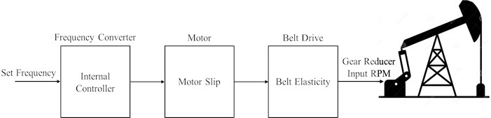
The first element of the surface system is the frequency converter, which powers the electric motor and rotates through the belt to drive the gear reducer’s input shaft (Fig. 3). At a certain power rating of the electric motor, it is necessary to use a frequency converter, due to the needed limitation of the inrush currents at the startup. Besides a field orientated closed-loop controlled operation also a higher motor dynamic can be achieved compared to a direct grid-connected motor. A belt connects the electric motor and the gear reducer intake shaft, causing additional damping.

Fig. 3Surface system

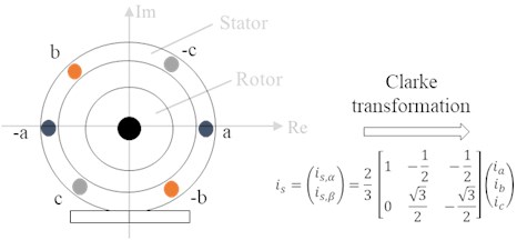
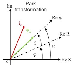
A physical model of the induction motor is used for modeling. The utilized motor and frequency converter types are known, but the applied control parameters not. To overcome this problem a fundamental wave model for the air gap flux of the electric motor is applied and combined with a standard control loop. The three-phase system of the electric motor is transformed via Clarke and Park transformation into a two-phase system, which is rotating aligned with the rotor flux space vector.

Fig. 4a) Representation of the induction motor windings. The current through the windings is transformed via a Clarke transformation into a 2 phase system; b) a Park transformation is applied to have a rotating reference frame. (S: stator coordination system, R: rotor coordination system, ψ rotor flux orientated coordination system; α=ϱ+φ)

a)

b)

The angular velocity $\omega$ of the rotor is:

5

$\omega =\frac{\dot{\phi }}{p},$

where $p$ is the number of pole pairs of the motor and $\dot{\phi }$ is the change of the electrical angle. To simplify the equations the main inductance $L_h$, the stator stray inductance $L_{\sigma ,S}$, the rotor stray inductance $L_{\sigma ,R}$, the stator winding and supply cable resistance $R_S$ and the rotor resistance $R_R$ are used to form the following terms. The index $S$ stands for stator and $R$ for the rotor:

6

$L_R=L_{\sigma ,R}+L_h,$
$L_S=L_{\sigma ,S}+L_h,$
$L_{\sigma }=\frac{\left(L_S{L}_R-{L_h}^2\right)}{L_R},$
$R_{\sigma }=R_s+{\left(\frac{L_h}{L_R}\right)}^2{R}_R.$

The space vector ${i_s}^{\psi }$ is described by Eq. (7), where $\psi$ is the reference frame:

7

${i_s}^{\psi }=i_{s,d}+j{i}_{s,q},$

where $d$ is the real and q the imaginary part of the space vector and $j$ is the imaginary variable. The main equation for describing the real and imaginary component of the electric stator current can be written in the following way:

8

${u_s}^{\psi }=R_{\sigma }{i_s}^{\psi }+L_{\sigma }\frac{{{di}_s}^{\psi }}{dt}+j\dot{\alpha }{L}_{\sigma }{i_s}^{\psi }+j\dot{\phi }\frac{L_h}{L_R}{{\mathrm{\Psi }}_R}^{\psi }-{\left(\frac{L_h}{L_R}\right)}^2\frac{{{\mathrm{\Psi }}_R}^{\psi }}{L_h}{R}_R,$

where $u_S$ is the applied stator voltage, $i_S$ is the stator current, $\dot{\alpha }$ is the angle between the real axis and the $\psi$ reference frame, and ${\mathrm{\Psi }}_R$ is the rotor flux. Due to the alignment of the coordination system to the real axis of the flux space vector, there is no imaginary component for the flux in the rotating frame (${{\mathrm{\Psi }}_R}^{\psi }={\mathrm{\Psi }}_{R,d}+j_0$). The differential equation for the real component of the flux is:

9

${\dot{\mathrm{\Psi }}}_{R,d}=\frac{R_R}{L_R}{(L_h{i}_{s,d}-\mathrm{\Psi }}_{R,d}).$

The angle $\dot{\varrho }$for the flux orientated reference frame is calculated with the following equation:

10

$\dot{\varrho }=\frac{1}{{\Psi }_{R,d}}\frac{R_R}{L_R}{L}_h{i}_{s,q}.$

The torque of the induction motor is calculated by Eq. (11):

11

$T=\frac{3}{2}p\frac{L_h}{L_R}{\mathrm{\Psi }}_{R,d}{i}_{s,q},$

where $T$ describes the torque of the electric motor. The delivered model to describe the induction motor electrically has an order of four. The developed control system consists out of two loops, one for controlling flux and one for controlling the speed of rotation. The control parameters were selected in a way to meet the behaviour of the measurements.

The motor shaft drives the V-belt pulley. The V-belt dampens the vibrations of the motor and drives the gear reducer input shaft. The V-belt damping effect is dependent on the properties of the V-belt and can be modeled by a combination of a transitional spring and a transitional damper [22]. A detailed analysis of the V-belt behavior was presented by Xing and Dong [23]. The V-belt behavior is described by two partial differential equations, one for the motor sheave pulley and another one for the gear reducer sheave. The influence of the slide angle and the equivalent rotational inertia are considered.

The gear reducer output shaft drives the pump jack, which the four-bar linkage system can describe geometry. John Svinos introduced a set of equations that allow the kinematic analysis of any component within the problem, for Conventional, Mark II and Air Balanced Units [24], which are used in the presented model. The angular velocity of the crank $\dot{{\theta }_2}$ is the basis of the pump jack’s dynamics evaluation. The walking beam movement and the polished rod behavior are depending on the crank’s angular velocity. Inertia effects of the pump jack and the counterweight are calculated based on that. The polished rod position $P_{PR}$ polished rod velocity $V_{PR}$, and the polished rod acceleration $A_{PR}$ is the linkage of the surface model with the downhole model:

12

$P_{PR}=A\left({\theta }_4-\frac{\pi }{2}-\delta \right),$

13

$V_{PR}=A{\dot{\theta }}_4,$

14

$A_{PR}=A{\ddot{\theta }}_4,$

where $A$ represents the distance between the walking beam bearing and the front of the horsehead, ${\theta }_4$ is the walking beam angle, and $\delta$ represents a pump jack geometry parameter. The torque factor $TF$ (Eq. (15)) is used to convert the polished rod load $F_{PR}$ into torque at the gear reducer’s output shaft $T_{load}$ (Eq. (16)) [25]:

15

$TF\left({\dot{\theta }}_2\right)=\frac{V_{PR}}{{\dot{\theta }}_2},$

16

$T_{load}=TF.F_{PR}.$

3.2. Downhole system

The downhole system accounts for the dynamics of the sucker rod string and the pump. A so-called transfer function is used to describe the rod string’s behavior, where the pump behavior represents the load boundary condition and the polished rod movement, representing the displacement boundary condition. In history, several transfer function types have been developed, where most of them are based on the viscous damped wave equation, introduced by S. G. Gibbs in the 1960ies [26]:

17

$\frac{\partial ²u}{\partial t²}=a^2\frac{\partial ²u}{\partial x²}-\frac{\pi av}{2L}\frac{\partial u}{\partial t},$

where $u$ is the displacement in the $x$-direction along the rod string, t is the time; a is the velocity of sound in the sucker rods, $x$ is the observed position, $v$ is a dimensionless viscous damping coefficient, and $L$ is the total length of the sucker rod string. The nature of the viscous damped wave equation comes along with some limitations. The second-order damped partial differential equation (Eq. (17)) accounts for the stresses in the sucker rod string, inertia effects, and fluid friction in vertical wellbores. Neither wellbore trajectory nor Coulomb friction is considered. As a result, the viscous damped wave equation’s application is limited to vertical wellbores, except some modifications or a workaround is considered.

Many scientists have used the work of Gibbs as a basis for their research [27], who have reported valuable results. The standard solution method is the finite difference method [26], [28], [29], [30], [31], [32], [33], [34]. The here shown model uses the finite differences method to solve the viscous damped wave equation. The rod string is divided into equal element length increments $\mathrm{\Delta }x$ and the time is discretized into increments of $\mathrm{\Delta }t$. The maximum rod element length should be between 50 and 100 meters to achieve a good result quality. $\mathrm{\Delta }t$ is chosen according to the Courant–Friedrichs–Lewy (CFL) condition [35], which indicates that the sound wave has to pass the length increment $\mathrm{\Delta }x$ at least in the time increment $\mathrm{\Delta }t$ Eq. (18). Literature indicates that three pumping cycles are sufficient to eliminate the initial start-up effects [28]:

18

$CFL=\frac{a\mathrm{\Delta }t}{\mathrm{\Delta }x}.$

The finite differences scheme can be visualized as a two-dimensional grid of displacement information. Fig. 5 shows the scheme for the sucker rod pumping system. The $x$-direction represents the time $j$, whereas the $y$-direction represents the space $i$. At the position $i=$ 1, the polished rod is situated, and at $i=m$, there is the downhole pump. Time step $j=$ 1 indicates the start and $j=n$ the end of the simulation. The constant parameters of Eq. 17 are summarized in constant $c_1$ (Eq. 19) and $c_2$(Eq. 20):

19

$c_1=\frac{\pi av}{2L},$

20

$c_2=a^2.$

Eq. (17) can be discretized by using the finite forward difference in time for the first derivative Eq. (21) and the central finite differences in time Eq. (22) and Eq. (23) space for the second derivatives:

21

$\frac{\partial u}{\partial t}\approx \frac{u_{i,j+1}-u_{i,j}}{∆t},$

22

$\frac{\partial ²u}{\partial t²}\approx \frac{u_{i,j+1}-2u_{i,j}+u_{i,j-1}}{∆t^2},$

23

$\frac{\partial ²u}{\partial x²}\approx \frac{u_{i+1,j}-2u_{i,j}+u_{i-1,j}}{∆x^2}.$

Through the use of Eq. (19) to Eq. (23) and a rearrangement to express the displacement $u_{i,j+1}$ at the requested time step, the discretized equation Eq. (17) can be written as Eq. (24):

24

$u_{i,j+1}=\frac{\left(2∆x^2+c_1∆t∆x^2-2c_2∆t^2\right).u_{i,j}-∆x^2.u_{i,j-1}+c_2∆t^2{u}_{i+1,j}+c_2∆t^2{u}_{i-1,j}}{(1+c_1∆t)∆x²}.$

Eq. (24) combines the displacement information of four points to determine the displacement information of the requested point. This so-called finite differences stencil at center $u_{i,j}$ is moved through the grid, starting from the node $u_{\mathrm{2,2}}$ downwards in space direction. When the final space node is reached, the stencil continues at the next step.

Fig. 5Finite differences scheme for the sucker rod pumping system

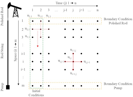
Fig. 5 indicates the necessity of two initial and two boundary conditions. The initial conditions define the displacement information at all space nodes for the first two time steps. The simulation starts from the static condition; thus, initial displacement Eq. (25) and velocity v are equal to zero:

25

$u_{i,1}=0.$

The backward finite difference is used to define the node velocity Eq. (26), representing the node displacement gradient:

26

$v_{i,j}=\frac{u_{i,j}-u_{i,j-1}}{∆t}.$

This representation implies that the first two time steps’ velocity equals zero Eq. (27):

27

$v_{i,2}=\frac{u_{i,2}-u_{i,1}}{∆t}=0\to u_{i,2}=u_{i,1}.$

The surface boundary condition is given by the polished rod’s movement and defines the displacement at nodes $u_{1,j}$. The pump boundary condition $u_{m,j}$ is defined by the pump load. One needs to distinguish between up-and-downstroke and the fluid load transfer between tubing and sucker rods. At the beginning of the upstroke, the rods' fluid load is taken from the anchored tubing. The rod string stretches, but there is no relative movement between the pump plunger and the tubing. As soon as the rod string carries the total fluid load, the plunger starts to move upwards. In addition to fluid load, velocity-dependent forces and acceleration forces start to act on the plunger Eq. (28):

28

$u_{m,j}=u_{m-1,j}-\frac{W}{E{A}_{rod}}∆x-{K_{v}v}_{plm,j-1}-K_a{a}_{plm,j-1},$

where $W$ is the fluid load, $E$ is Young’s modulus of the rod material, $A$ is the rod cross-section, $K_v$ is the proportional velocity coefficient, $v$ is the plunger’s velocity, $K_a$ is the proportional acceleration coefficient, and a is the plunger’s acceleration. At the top dead center, the fluid load is handed over again to the tubing string, the standing valve closes, and the traveling valve opens. Again, there is no relative movement between the tubing string and the pump’s plunger during this procedure. During the plunger’s downstroke, buoyancy, velocity, and dependent acceleration forces are acting on it Eq. (29):

29

$u_{m,j}=u_{m-1,j}-\frac{B}{E{A}_{rod}}∆x-{K_{v}v}_{plm,j-1}-K_a{a}_{plm,j-1}.$

B represents the buoyant force, the displacement trend for the investigated nodes is the key to further evaluating rod string loads, velocities, stresses, production rate, and power requirements. The polished rod load $F_{PR}$ can be evaluated by calculating the top section's rod stretch Eq. (30). The model itself does not account for the gravitational force $F_G$ of the rod string and is added during the post-processing step:

30

$F_{PR}=\frac{u_{1,j}-u_{2,j}}{∆x}E{A}_{rod}+F_G.$

The damping coefficient is the only unknown when using the viscous damped wave equation as a transfer function. A low damping coefficient results in unusual fluctuations of the dynamometer card, whereas a high damping coefficient causes a ballooning of the dynamometer card. An ideal damping coefficient is in between and typically in the range of 0.1 [36].

The numerical model was used to develop the frequency-elastic drive mode prior to the field test and to understand the effects, caused by the manipulation of the $C_T$ and $C_K$ parameters.

4. Experiment: frequency - elastic drive mode field test

The field-tested sucker rod pumping system is installed in a vertical wellbore. The wellbore is equipped with an 800 meter long anchored 3 1/2 in tubing string. The downhole pump is a 30-225-RHAC-18-4 SRABS pump type [37], set at 800 m and operated with a conventional VSD drive at 8.57 strokes per minute. The rod string comprises 280 m of 1” rods grade D, 490 m of 7/8” rods grade D, and 30 m of 2” sinker bars. The recorded fluid properties are 25° API oil gravity, a 113 Pa/m gas gravity, and 98.8 % water cut. Under regular operation the dynamic fluid level is at 475 m from the surface, a casing head pressure of 11 bar and a tubing head pressure of 8 bar are seen. The pump’s gross production rate is 90 m³/day. The pump jack is a conventional one of type C-320D-256-144.

The selected pump jack is equipped with a high-speed measurement system, which allows the recording of sensor readings at a frequency of 5 kHz. For the field test, the frequency converter current and voltage, the crank speed, the polished rod movement, and polished rod load have been measured.

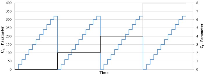
The frequency-elastic drive mode was tested for the set frequencies of 40, 45, 50, 51, and 55 Hz. Several $C_T$ and $C_K$ parameters were tested for each set frequency. $C_T$ was chosen in the range between zero and eight with two as increments. For each $C_T$ parameter, 12 $C_K$ parameters in the range between 0 and 320 with an increment of 30 were tested. Fig. 6 summarizes the test procedure regarding the parameters for one frequency.

Fig. 6CT and CK parameters tests for each frequency – CT was defined to start with zero and remain at this value until all CK were tested. As a next step, CT was increased by two and again all CK were tested. After this procedure was finished all parameters the next frequency was applied

5. Results: field test

The recorded data are used to evaluate the actual strokes per minute, the polished rod displacement, and the energy consumptions at the polished rod and frequency converter. Fig. 7 and Fig. 8 compare the polished rod movement and the dynamometer cards for a set frequency of 50 Hz and several $C_T$ and $C_K$ parameters.

A low $C_T$ parameter and a moderate $C_K$ parameter results in a slowing down of the pump jack during the upstroke and a reduction of the peak velocities. An increase in the $C_T$ parameter reduces the effect of the $C_K$ parameter. The dynamometer cards indicate a reduction of the peak polished rod load and an increase of the minimum polished rod load for the frequency-elastic drive mode. The magnitude is depending on the selected parameters. The area of the dynamometer cards slightly reduces with the increase of the parameters, indicating an increase in the system efficiency. Nevertheless, an increase in the system dynamics can be seen.

Fig. 7Polished rod movement – frequency-elastic drive mode

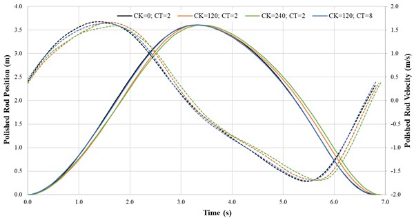
Fig. 8The dynamometer card comparison of the standard (black line) and frequency-elastic drive modes indicate a reduction in load and energy consumption. Nevertheless, the dynamics in the downhole system increase. The degree is dependent on the selected parameters. A CT parameter equal to two and a CK parameter of 120 shows fewer dynamics than a CT parameter equal to two and a CK parameter of 240. CT reduces the effect of CK and CT equal to 8 and CK equal to 120 shows fewer dynamics than the previous parameters

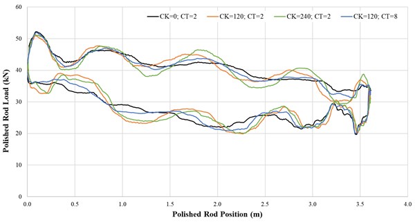
Fig. 9The SPM is influenced by the CT parameters. The influencing range is about 0.3 SPM for CT parameters between 0 and 8

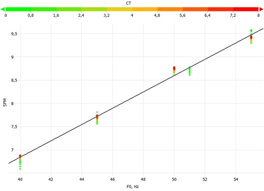
The change in frequency, $C_T$, and $C_K$ parameters influenced the pumping speed, the loads, and the energy consumption of the pumping system significantly. Fig. 9 presents the actual strokes per minute for the set frequency and the tested $C_T$ parameters. For the frequency of 51 Hz, just the $C_T$ parameter of zero was tested. The results show that the actual number of strokes per minute decreases with increasing $C_K$ parameters but increases with increasing $C_T$ parameters.

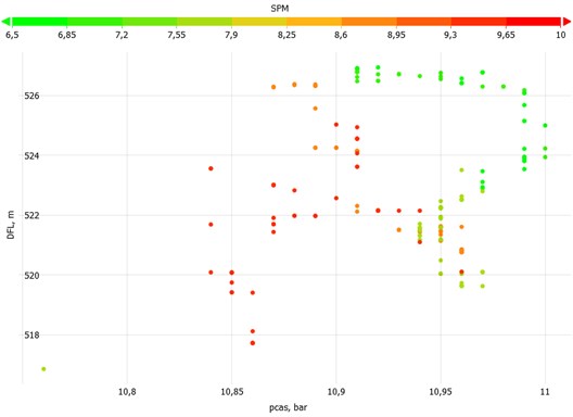
The pumping speed influences the dynamic fluid level (DFL) in the annulus, the tubing ($p_{tub}$), and casing ($p_{cas}$) head pressure (Fig. 10 and Fig. 11). The dynamic fluid level is related to the inflow performance of the reservoir. An increase in the pumping speed results in a slight increase in the tubing head pressure, a drop in the casing head pressure, and dynamic fluid level.

Fig. 10The field tests were performed for a pumping speed range of 6.5 to 9.5 SPM. The tubing head pressure changed from 7.05 bar to 7.5 bar and the fluid level dropped from 527 m to 519 m above the pump intake

Fig. 11The increase in pumping speed resulted in a marginal reduction of the casing head pressure from 11 bar to about 10.85 for 9.5 SPM

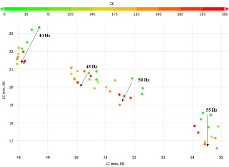
Significant dependencies of the peak polished rod load ($L{C}_{max}$) and the minimum polished rod load ($L{C}_{min}$) have been seen not only for a change in the set frequency but also for a change in the $C_T$ and $C_K$ parameters. A substantial increase in the peak polished rod load from 48 kN for 6.5 SPM to 55 kN for 9.5 SPM occurred. The data indicate a parabolic relationship between peak polished rod load and pumping speed. Fig. 12 and Fig. 13 present the peak polished rod to load on SPM behavior for the $C_T$ and $C_K$ parameters.

Fig. 12This plot presents the peak polished rod load recordings for CT equal to zero and changing CK. An increase in the CK parameter reduces the peak polished rod load and the pumping speed for the set frequencies of 40, 45, and 51 Hz, whereas an increase in pumping speed and peak polished rod load was seen for the set frequency of 55 Hz. In total, the peak polished rod load increased by 7 kN

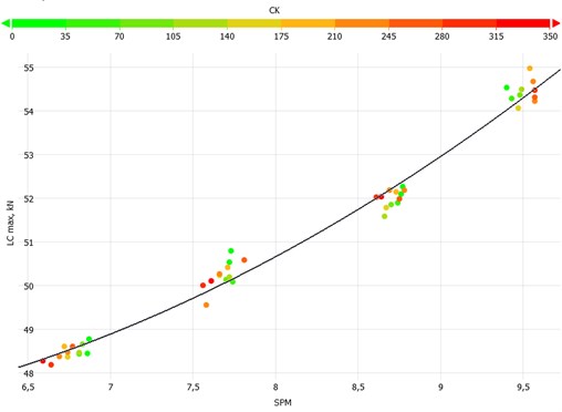
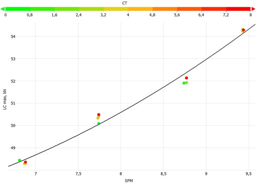
Fig. 13This plot presents the recordings for CK equal to 60. The increase of the CT parameter increases the pumping speed and an increase in the peak polished rod load for all set frequencies

A drop in the minimum polished rod load has been seen for the increase in the pumping speed in general. Fig. 14 and Fig. 15 summarize the cross plots and the linear trend for defined $C_T$ and $C_K$ parameters.

Fig. 16 shows the cross plot of minimum and peak polished rod load for the $C_T$ parameter equal to two. The trend towards lower polished rod load can be seen for the increase in the $C_K$ parameter.

In contrast, Fig. 18 presents the polished rod energy consumption and frequency converter energy consumption for all $C_T$ parameters. It shows that the polished rod energy consumption decreases with the increase of the $C_K$ parameter for all set frequencies. But more importantly, the frequency converter energy consumption increases slightly for 40 and 45 Hz, but drops for 50, 51, and 55 Hz. This is the result of the pump jack dynamics.

Fig. 14This plot presents the peak polished rod load recordings for CT equal to zero and changing CK. An increase in the CK parameter reduces the minimum polished rod load and the pumping speed for the set frequency of 40 Hz. An increase in pumping speed and the minimum polished rod load was seen for the set frequency of 55 Hz. For 45, 50, and 51 Hz no trend can be identified

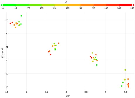
Fig. 15This plot presents the recordings for CK equal to 60. The increase of the CT parameter increases the minimum polished rod load for the set frequency of 40 Hz. For the set frequencies of 45, 50, 51, and 55 Hz the minimum polished rod load drops by the increase of CT. In total the minimum polished rod load dropped by 6 kN

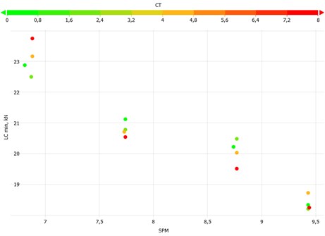
Fig. 16Cross plot – minimum and peak polished rod load

The energy consumption of the pump jack was evaluated at the polished rod ($E_{mpr}$) and the frequency converter ($E_{mo}$). Fig. 17 shows the cross plot of polished rod energy consumption on the y-axis and the frequency converter energy consumption on the $x$-axis for all $C_K$ parameters. The increase in the $C_T$ parameter results in a slight reduction of the frequency converter energy consumption and the polished rod energy consumption for low set frequencies. For higher set frequencies the energy consumption increased.

Fig. 17Cross plot of polished rod energy consumption and frequency converter energy consumption for all CK parameters

Fig. 18Cross plot of polished rod energy consumption and frequency converter energy consumption for all CT parameters

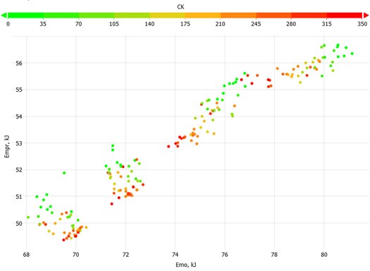
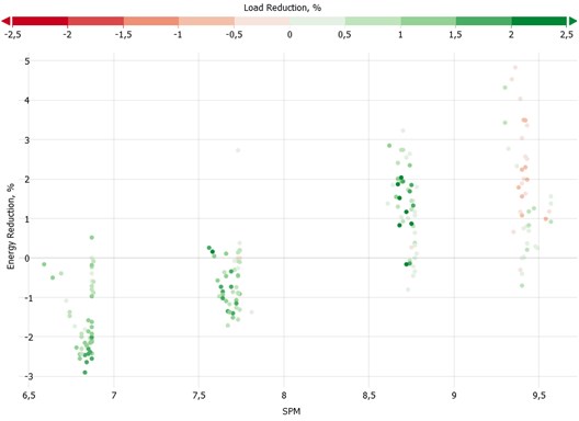
Fig. 19 indicates the energy consumption reduction based on the actual pumping speed. For the given system the frequency elastic drive mode shows a significant energy reduction potential of up to 5 percent for a pumping speed above 8 strokes per minute. Below that more energy is required to operate the system. Nevertheless, the color bar indicates the peak polished rod load reduction. The frequency elastic drive mode reduces the peak load for low and moderate pumping speed but causes an increase for high pumping speed. As a result, for the given pumping system there is the optimum range of application.

The evaluation of the field test results has shown that the application of a low $C_T$ parameter in combination with a high $C_K$ parameter influences the pumping systems towards energy saving and load reduction. The frequency elastic drive mode yields the best results for the field-tested pumping system and optimized parameters in the pumping speed range between 7 to 10 strokes per minute.

Fig. 19Energy consumption reduction based on actual pumping speed

6. Discussion: model evaluation

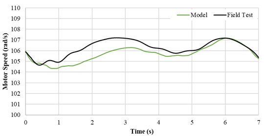
The numerical model, used to develop the frequency-elastic drive mode, was built by 50-meter space increment and 5 milliseconds of time increment. The actual verification of the model with the field data was performed for regular pumping operation without the novel frequency - elastic drive mode algorithms after the development. Fig. 20, Fig. 21, Fig. 22, and Fig. 23 present a detailed comparison of the numerical model results and the field test recordings. The polished rod displacement comparison shows an excellent match. The surface dynamometer card comparison and the motor power consumption show a good match. Nevertheless, some discrepancies can be seen.

The motor shaft speed was 107 rad/s slightly higher than the simulation result with 106 rad/s at the time step of 3 seconds.

Fig. 20Polished rod position comparison

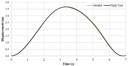
Fig. 21Dynamometer card comparison

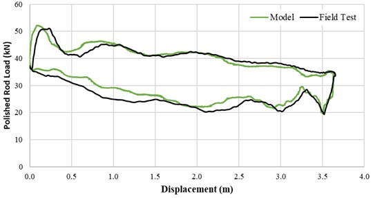
Fig. 22Motor power consumption comparison

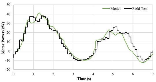
Fig. 23Motor shaft speed comparison

7. Conclusions

The research has shown that software adjustments at the drive controller enable an improvement in the energy efficiency of the sucker rod pumping system. By manipulation of the set frequency of the frequency converter with a time constant and a proportional constant, an optimized pumping system motion is achieved. The time constant is responsible for data filtering, whereas the proportional constant scales the adjustment of the set frequency based on the load at the electric motor.

A numerical model has been developed and used to verify the frequency – elastic drive mode in parallel to an extensive field test. The numerical model accounts for all relevant components of the sucker rod pumping system and is verified by the field test recordings. A detailed analysis of the field test recordings resulted in the fact that the effect of the frequency-elastic drive mode is significantly influenced by the sucker rod pump configuration and operation conditions. The field test was performed on a vertical wellbore, equipped with a 800 m long rod string and a 30-225 RHAC SRABS pump. For the system, tested in the field, a significant energy consumption reduction of up to 5 percent and a polished rod load reduction of 3 percent was achieved.

The model is a convenient way to perform a parameter study and further investigate the effects of the frequency-elastic drive mode for other well configurations before applying the novel frequency-elastic drive mode in the field on other wells.