Abstract
Three new algorithms for synthesizing control for the model of an electrohydraulic disk brake system are presented, which are based on the synergetic control theory. The first algorithm is developed relying on the classical method of analytical design of aggregated regulators in an assumption of a completely defined object. The second algorithm represents an algorithm of nonlinear adaptation on a target manifold and is designed for an object with a nonrandom disturbance in the control channel. The third algorithm takes account of the random disturbance in the discrete description of this object and rests on the strategies minimizing the dispersion of the output macrovariable. The results of a comparative numerical simulation of the three control algorithms are presented and the recommendations concerning the selection of the regulator parameters are formulated depending on the level of systematic disturbances and random noise.
1. Introduction
An increased interest is demonstrated in the system synthesis algorithms relying on the physical control theory and its implementation methods not only due their “closeness” to the natural properties of objects but also for a reason of the most “delicate” and energy-saving intrusion into their behavior to achieve the target and desirable properties [1]-[3].
The purpose of this study is to design an asymptotically stable and robust synergetic [1] control over an electrohydraulic disk brake for a rail car wheel set; its initial model was of the 10-th order and later was reduced to the 4-th order (which is sufficient for control synthesis due to a synergetic interconnectedness of the object’s coordinates). The mathematical description used here was proposed at the Institute for Power Drives and Control at Aachen University (IFAS RWTH Aachen University, Germany) and is termed as a self-energizing electrohydraulic brake (SEHB) [3].
Despite the fact that the problem has been discussed for a long time, today there is no control with satisfactory properties for the case of increased or decreased braking power. Note that in the open-loop condition at u=0 the object is unstable.
The analogs of control algorithms over this object are the algorithms based on the proportional-integral-differential (PID) controller and on the method on feedback linearization (MFL) [3]. The limitation of the former is the oscillatory braking character, which results in the wear of the mechanical section of the brake. The costs of control in the latter method are by 4-11 factors lower compared to those in the system with a PID-controller, but it demonstrates poorer properties at the critical values of the braking coefficient (parameter), which is undesirable in terms of practical implementation of this algorithm.
In this work we propose a pioneering alternative synergetic approach to the process of synthesizing a nonlinear regulator for such an object; one of its advantages is the energy-saving effect of the control system, which is accounted for by the correct use of the phenomenon of self-organization of the object after the set target has been achieved.
The result presented here is theoretical; it consists in an analytical design of a regulator compensating for the unknown restricted disturbances over the control channel.
1.1. Technical description of a control object
According to the technical description of a SEHB object [1]-[3] (Fig. 1), it includes a friction-type brake using the friction power as an energy source for generating a new braking power by transferring the electrohydraulic energy. A dual-action hydraulic cylinder, referred to as a base cylinder here, connects the break support with the railroad car structure, fixing the hydrocylinder piston between two columns of the brake liquid. In the case of braking, the friction force acts on the base cylinder piston, causing a pressure change in its cavities. The liquid pressure in the high hydraulic level does not practically change due to an expansion tank used in the system, whose volume is much larger than the total volume of the hydraulic circuit line and the base cylinder cavity; a spool valve connects the hydraulic lines with the hydraulic motor cavities. In the case where the direct connection of hydraulic lines is active (increasing braking power), the liquid is pumped into the piston cavity of the hydraulic motor, while its rod end is connected to the low-pressure line.
Fig. 1Schematic representation of a SEHB
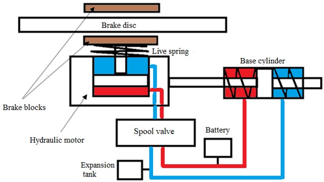
Note that the selected ratio between the total and the annulus area of the differential cylinder piston gives rise to a self-excited process of the brake power increase. If the reverse connection of hydraulic lines is active (decreasing braking power), then the piston cavity is connected with the low-pressure line and the liquid from the supply pressure line is delivered to the rod end.
A detailed description of the features of the functioning of the considered SEHB control object is considered in publications [1]-[3], here we will be interested only in the formal description of the behavior of its mathematical model in the state space.
1.2. Mathematical apparatus of the synergetic approach for the design of nonlinear regulators
The ADAR method, implemented in what follows, includes the physical aspects of the controlled object via special invariants whose description is a mathematical manifold with an attractive property; the synthesized regulator is robust and satisfies the least action principle.
Let us formulate the following requirements [4]-[7] to the initial description and the necessary a priori information for applying the procedure of synthesizing an ADAR-control:
а) initial mathematical description of the control object is given by a system of ordinary differential equations or a system of difference equations for continuous and discrete control problems, respectively;
b) availability of a globally stable target system for initial model, which satisfies the target analytically set invariant , , where , is the continuously differentiated function, , ;
c) boundedness of all solutions of the initial system;
d) stabilizability of all object’s trajectories in the neighborhood of ;
e) implementation of the control system synthesis in the state space in the absence of any restrictions on the controls linearly included into the right-hand parts of the object’s descriptions.
f) ADAR-control provides a solution to variational problems or for continuous and discrete description of the object, respectively:
where the parameters , , are the settings of the regulators.
2. Control problem statement
Let the mathematical models for the description of two operating modes of the object be those with increasing and decreasing braking powers, respectively. Due to a certain symmetry of the mathematical models, it is enough to consider one of them only, for instance, a system of equations for increasing braking power with a purpose of obtaining an algorithm for designing the form of the control action on the target manifold principles and the method of analytical design of aggregated regulators (ADAR) [4], [5] given by:
Above, the control object variables and parameters have the following notations (see, e.g., [3]). The variables are: – load pressure; – supporting pressure; – control valve spool velocity; – control valve spool movement; – input solenoid voltage of the sliding spool valve (control valve input) realizing the goal achievement , , where is the set value (problem of stabilization at or tracking at ); quantities , are the known coefficient and the parameter depending on the friction coefficient , respectively; , , are the valve parameters; is the piston area ratio of the brake actuator; is an unknown bounded function, and is the liquid pressure in the low-pressure line.
The article presents two algorithms for designing control in the state space of the unstable object with a different physical nature of disturbances. Let us name them conditionally NAD (Nonlinear ADaptation algorithm for a nonrandom object [7]-[9]) and NAS (Nonlinear Adaptation algorithm for a Stochastic object [10]). Note that both algorithms are correct extensions of the classic ADAR-algorithm [7], [10] (see Appendix A1).
For the sake of readability and brevity, we denote the original description as , giving the indices or depending on the design algorithm under consideration.
It is required:
1) to design a system of control for the model of a nonlinear 4-th order object (1); the quality functional of the sought-for control contains the requirements both to the target system , and to the transient process dynamics ; we will refer further to the form of the variational problem as ;
2) to be convinced in the performance of the resulting control system using the model data reported in [1]-[3]; and
3) to study the properties of the regulator robustness in the off-model (off-design) conditions.
It is also assumed that the classic conditions required for the correct application of ADAR must be fulfilled.
Let us supplement the above-formulated conditions a)-f) with the following items:
1) disturbance is an unknown, bounded and continuous function of time, and the range of its values does not result in any violation of the above-formulated conditions a)-с);
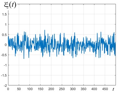
2) simulation of disturbances relies on the results presented elsewhere [8], demonstrating that a) continuous functions can be described as partial solutions to differential equations; b) disturbances can have a wave representation.
3. Nonlinear adaptation algorithm for designing control including nonrandom disturbances
Derivation of a control system based on the classical method (see Appendix A) is a special case of the NAD-algorithm. Therefore, let us dwell on the last algorithm in detail.
3.1. Basic provisions of the NAD-algorithm
It is well known that the use of the ADAR-synthesis guarantees robust properties to the designed regulator, ensuring a suppression of the external and parametric disturbances. Given this, the disturbances can be modeled as piecewise-constant functions in the differential equations of the object, which include controls, and the system of equation is supplemented with the integrator equations [7], [9].
In this case, the algorithm for synthesizing the required control stabilizing the target variable , will be implemented by the following steps.
1. Phase space extension or transformation of the initial description into a closed system, for which a classical ADAR-synthesis is already possible. We obtain a system of the form
where is the designed regulator parameter.
2. Euler-Lagrange equation for the functional only, where would ensure the following form of the regulator structure:
3. Decomposition of (2) on the set of states , would yield a system of equations:
4. Euler-Lagrange equation for the functional only, where , would ensure the following form of the regulator :
5. Decomposition of Eq. (4) on the set of states , would yield a system of equations:
6. Solution of the variational problem with a target invariant of a special form , , ( – one more system parameter) is provided by the Euler-Lagrange equation , from which, including Eqs. (6), find an expression for variable :
Having determined the partial derivatives from (5), (7) and combining together Eq. (3), we obtain the final system with the regulator (see Appendix A2).
Statement 1. Control , if any, ensures an asymptotic stability for the controlled object Eq. (1) in the neighborhood of ,
Proof of Statement 1 is constructive and immediate from the NAD-algorithm of control system synthesis for Eq. (1) (see, e.g., [7]).
4. Nonlinear adaptation stochastic algorithm for designing discrete control
4.1. Problem statement of stochastic discrete NAS-control
Represent the description of object Eq. (1) in accordance with the Euler scheme given by
where is the random bounded function and parameter is the discretization value of the continuous description Eqs. (1).
As above, we will denote the original description as , , ,
The problem of stochastic control will be formulated as follows: it is required to design a control system for a stochastic object Eqs. (8), providing:
1) an asymptotically stable on average achievement of the target , , where is the sign of a mathematical expectation of a random value of ;
2) a minimum to the quality functional ;
3) a minimality of dispersion of the output macrovariable and of all intermediate macrovariables appearing in the implementation of the ADAR-synthesis hierarchical subproblems (subgoals) of the control design).
As far as random noise in the description Eqs. (8) is concerned, assume that is a sequence of independent evenly distributed quantities with the properties of , ; is a certain constant interpreted as a noise damping coefficient; .
Restrictions on the choice of command variables are as follows [10], [11]:
1) control strategies are selected from the class of discrete ADAR-controls;
2) those strategies, for which the value of the control variable is a function of the previous states and controls, are taken into consideration: , ;
The peculiarities of the discrete analog of the ADAR-synthesis are accounted for by the following [5] proposition.
Statement 2. The minimum of the average value of functional is achieved by solving the discrete analog of the Euler-Lagrange equation , , for which case the relationship between the parameters , is expressed via the formula [5].
4.2. Basic provisions of the NAS-algorithm
The algorithm for designing a stochastic control on a target manifold is represented by the following actions.
Step 1. Derive the control structure , relying on the classical discrete variant of the ADAR method at fixed random noise.
Step 2. Take the operation of conditional mathematical expectation , where .
Step 3. Decompose description Eq. (6) taking into account the discrete equations. Substitute the found control into the expression . Find the dependence as a function of the observations for the sake of exclusion of variable from expression . The synthesis of a discrete stochastic regulator is completed.
Statement 3. Control , if any, ensures an asymptotic stability for the object of control Eq. (6) on average in the neighborhood of , and a minimal dispersion of the output macrovariable .
Let us apply the NAS-algorithm to find the stochastic regulator for Eqs. (8).
1. Derivation of a control system structure. We fix the random functions , and perform a discrete ADAR-synthesis [4] for the control object Eqs. (8) with control quality functional , , denoting the control of this step as . Enumerate the steps of the discrete ADAR-synthesis for object Eq. (8).
A subscript in Eq. (9) indicates a substitution of the right-hand sides in Eq. (9) for , ; , .
Then decompose system Eq. (8) on manifold or :
Afterwards, for the control object (10) with the control quality functional , , from the Euler-Lagrange equation obtain:
Decomposition of Eq. (10) on the manifold , would yield a system of equations:
Perform a discrete ADAR-synthesis for the control object Eq. (12) with control quality functional , , :
The outcome of the first step is the control structure (at fixed noise) as a combination of Eqs. (9), (11) and (13).
2. A control for the object under the conditions of unknown (restricted) noise is sought for in the form of a conditional mathematical expectation , considering Eqs. (9) as follows:
3. Determination of an estimate of the random function as a dependence on observations. Let us use the expression for control Eq. (14) including the initial description Eq. (8) in the left-hand part of the functional expression: . Considering the above relation, obtain control in an explicit form:
The final description of the stochastic control system involves a combination of Eqs. (8), (11), (13) and (15):
Here the values , , , , are the settings of the regulator that provide the required quality of transient processes.
It is important to note that the parameters , are directly proportional to the duration of achieving the target manifold , for system Eq. (16).
4.3. Results of numerical simulation of three control algorithms under design and off-design conditions
Numerical modeling (Figs. 2-3) of the designed control systems (see Appendix A2) has been performed in the Matlab/Simulink environment using the following parameter values [3]: 15820; 35319.96; 628.3; 394760.89; 0,609; 500000; 10-3; 10-4; 2⋅10-4; 394760.89; 0.7; 0.4; 0.4, where is the valve damping coefficient; is the friction coefficient; is the target value of .
Fig. 2Behavior of the target coordinate x2t, Pa of the SEHB-objects (1) under different disturbances
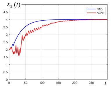
a); 3.97×10⁻²; 1.83×10⁻³
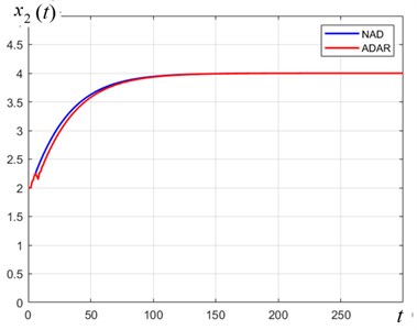
b) 30; 1.3×10⁻³; 9×10⁻⁴
Fig. 2 presents the curves of variation of the target variable according to the ADAR and NAD controls, respectively; they imply that a) the control target is being achieved; b) the transient process exhibits an acceptable quality; c) under conditions of constant disturbances, both algorithms are equally effective. The control energies are designated as and , respectively.
Fig. 3Comparison of the quality of transient processes of controllable variable x2t, Pa of the SEHB-object in response to controls uADAR, uNAD and uNAS, respectively
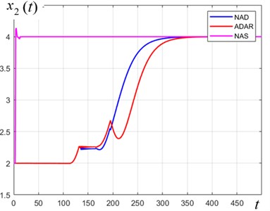
a) 1.36×10⁻², 1.39×10⁻², 19.3
b) Noise is normal
As follows from the above results (Figs. 2-3), the ADAR- and NAD-controls are comparable with respect to the quality of transients and the energy spent under constant disturbances.
If the disturbance s function is harmonic, then the use of the NAD control is clearly preferable. For large values of the “noise-to-signal ratio” indicator, the control efficiency will be in favor of the NAD (or NAS)-control.
4.4. Results of numerical simulation of synergetic control algorithms and previously constructed regulators
It was noted above that one of the earlier constructed regulators for a SEHB object is a PID-regulator and the second regulator is based on the feedback-linearization algorithm [3].
Figs. 4(a), 4(b) and Table 1 suggest promising conclusions in favor of the synergetic approach to the control over such an object, which however, needs more detailed research using an object’s prototype and under the conditions of different practical implementations of the object (motor car, train) [12].
Fig. 4Comparison of the control quality indicators under random noise conditions
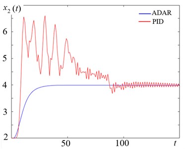
a) Transient processes of controllable variable , Pa (×105) of the SEHB-object in response to controls and , respectively
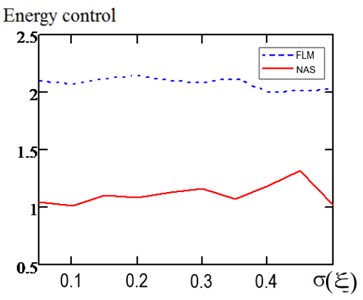
b) Comparison of the energies spent on control upon reaching the target values in conditions of normal random noises
The data are given for the spool damping parameter 0.4 and the friction coefficient of the brake pads 0.35.
Table 1Control quality indicators under random noise conditions
Regulator type | Average overshoot value along the coordinate | Average overshoot value along the u variable, % | Average control power, conv.un. |
ADAR | 0.7 | 1.5 | 0.4 |
NAD | 0.3 | 0 | 0.1 |
NAS | 1.6 | 0.1 | 1.2 |
PID | 5.8 | 9.2 | 15.2 |
FLM | 1.8 | 1.9 | 2.2 |
5. Conclusions
We have proposed three new algorithms for designing a control system, which bring a fourth-order nonlinear unstable SEHB-object described by a system of differential/difference equations to a target manifold.
The first algorithm, ADAR, is correct for a SEHB object of control without considering the disturbances, the second algorithm, NAD, is meant for compensating nonrandom disturbances, for the third algorithm, NAS, the design conditions are random disturbances.
All these algorithms have a common basis – they rely on the principles of the analytical design of aggregated regulators [4], [5] based on the synergetic control theory.
A common condition for application of the constructed control algorithms is the analytical setting of the target invariant in the form of a desired relationship between the state variables of the controlled object.
The results of a comparative simulation of the three algorithms constructed in this study under the design and off-design conditions among themselves and their comparison with other earlier constructed algorithms have been presented [1]-[3].
Summing up the simulated control systems, we argue that:
1) the algorithms for synthesizing regulators on a target manifold ensure robust properties of all three regulators (ADAR, NAD and NAS) under the conditions of different-type disturbances;
2) the algorithm based on nonlinear adaptation (NAD) has a clear priority with respect to the classical ADAR algorithm under the conditions of a physically acceptable level of disturbances of nonrandom and random types;
3) the NAS-control for “large” values of the random noise level has the least variation of the output variable compared to that of the NAD, ADAR and algorithms reported elsewhere [3];
4) the transient processes of the control systems under the conditions comparable with those reported in [3] at the same values of the friction parameter have the least dispersion;
5) the constructed synergetic regulators are characterized by lower energy costs (8 %-10 % in the model conditions) compared to two currently available control algorithms - the PID-control and the control designed using the feedback linearization method.
Further research should be focused on designing a NAS-algorithm in the space of observations, as the most generic among the available algorithms, aiming at reducing the dispersion of the output variable. In particular, the preliminary numerical experiments suggest that kernel smoothing of the target variablesin the regulator reduces the level of scatter of the transient processes.
References
-
M. Liermann, “Self-energizing Electro-Hydraulic Brake,” Ph.D. Thesis, Shaker Verlag, Aachen, 2008.
-
M. Liermann and C. Stammen, “Selbstverstärkende hydraulische Bremse für Schienenfahrzeuge,” Ölhydraulik und Pneumatik, Vol. 50, No. 10, pp. 500–507, 2006.
-
A. Starykh and M. Liermann, “Non-linear controller design based on the input-output linearisation method for a self-energising electro-hydraulic brake,” International Journal of Modelling, Identification and Control, Vol. 20, No. 1, p. 64, 2013, https://doi.org/10.1504/ijmic.2013.055914
-
A. A. Kolesnikov, “Introduction of synergetic control,” in 2014 American Control Conference – ACC 2014, pp. 3013–3016, Jun. 2014, https://doi.org/10.1109/acc.2014.6859397
-
A. А. Kolesnikov, Synergetics and Problems of Control Theory: Collected Articles. (in Russian), Moscow: Fismatlit, 2004.
-
A. A. Krasovskiy, “Problems of Control Physical Theory,” (in Russian), Automation and Remote Control, Vol. 1, pp. 3–28, 1990.
-
S. I. Kolesnikova, “Synthesis of the control system for a second order non-linear object with an incomplete description,” Automation and Remote Control, Vol. 79, No. 9, pp. 1558–1568, Sep. 2018, https://doi.org/10.1134/s0005117918090023
-
S. Johnson, “The theory of regulators to adapt to disturbances,” in Filtering and stochastic control of dynamical systems, Moscow: Mir, 1980, pp. 351–370.
-
A. A. Kolesnikov, New Non-Linear Flight Control Methods. (in Russian), Moscow: Fismatlit, 2013.
-
S. Kolesnikova, “Stochastic Discrete Nonlinear Control System for Minimum Dispersion of the Output Variable,” in Advances in Intelligent Systems and Computing, Vol. 986, Cham: Springer International Publishing, 2019, pp. 325–331, https://doi.org/10.1007/978-3-030-19813-8_33
-
K. J. Astroem and B. Wittenmark, Adaptive Control. New York, USA: Dover Publications, 2008.
-
M. Liermann, C. Stammer, and H. Murrenhoff, “Development of a self-energizing electro-hydraulic brake (SEHB),” in SAE 2007 Commercial Vehicle Engineering Congress and Exhibition, Oct. 2007, https://doi.org/10.4271/2007-01-4236
About this article

The reported study was funded by RFBR according to the research project No. 20-08-00747.
