Abstract
In response to the competing factors governing the operation of oil and gas facilities, i.e., the stringent safety and environmental regulations, and the challenging business environment that entails minimizing the running cost, a risk-based inspection (RBI) program became a vital part of all Asset Integrity Management (AIM) frameworks. The objective is to ensure asset mechanical integrity while optimizing the maintenance and inspection resources and minimizing production downtime. There are different risk models being used to manage operational risk for equipment. The decision-maker should be attentive to the subjectivity and reliability of the risk results to establish an adequate risk target that can achieve the ultimate goal of RBI by determining the cost-effective inspection and maintenance plan without compromising plant safety, integrity or reliability. This paper presents evaluations of the most quantitative RBI models through a case study from an offshore gas producing platform. A case study was implemented for topside equipment on an offshore platform. The study analyzed the impact of contributing factors to the probability of failure (PoF) model through a sensitivity analysis to quantify the reliability and subjectivity in the failure probabilities. A sensitivity analysis and comparison between both API consequence modelling methodologies (i.e., CoF level 1 and 2) were performed to manifest the reliability of risk results. The sensitivity analysis revealed the variance in the calculated risk and demonstrated that a risk target/threshold should be established based on the deployed risk model. Using the same risk target for different risk models cannot effectively define all equipment items that actually need more resources to mitigate the risk. And can result in omitting critical equipment which can jeopardize asset integrity and lead to major losses, or spend resources on unnecessary equipment.
Highlights
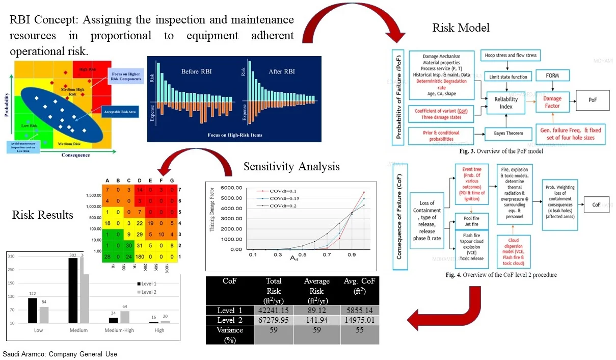
- Assigning the inspection and maintenance resources in proportional to equipment adherent operational risk will result in optimizing resources without compromising the equipment mechanical integrity. The challenge is establishing the risk tolerance/risk target to segregate high and low risk equipment.
- If the equipment operational risk was not estimated correctly and/or an adequate risk target was not established, the results will be either, overlooking some critical equipment, assigning maintenance and inspection resources to the wrong equipment or give a false feeling of safety which leads to relaxing important inspection and maintenance activities. These misleading results of RBI assessment can jeopardize the plant integrity and fail in achieving the main objective of RBI assessment.
- This paper critically discusses API 581 RBI model to evaluate the reliability and subjective of the risk calculations. The analysis was conducted through a case study at offshore platform. the case study included both API consequence models (i.e., level 1 & 2) and sensitivity analysis for the parameters contribute to the PoF calculations.
- The work presented in this paper revealed the need to develop more objective risk model especially for offshore platforms to address the unique features of consequence modelling.
1. Introduction
The challenging current global oil and gas business environment forces the industry to maintain production at lower costs, with higher quality and integrity to satisfy the more existing rigorous safety and environmental regulations. To encounter this challenge and achieve the highest profitability, [1] over the last decades the implementation of risk and integrity management approaches is prospering up. The conventional inspection plans (time-based inspection) do not give the desired flexibility, and do not allow cost-effective risk management [2-4]. Therefore, over the last decades, a risk-based inspection (RBI) methodology became the state of art of inspection planning approach/strategy to increase availability and reliability (minimizes unplanned shutdown); it allows flexible inspection intervals without jeopardizing equipment integrity; increases Inspection overall efficiency; eliminates inspection activities that don’t add value; increases safety; and provides a solid and traceable technical basis to justify inspection interval changes for regulators and being fully auditable process [4-6].
Because of the benefits RBI can provide, RBI became a vital part of any Asset Integrity Management (AIM) program, particularly in the oil and gas industry [8-10]. RBI seeks to ensure the mechanical integrity of static or fixed equipment of a production process; therefore, the assets can meet the performance requirements while optimizing inspection and maintenance resources. In focusing on risks and their mitigation, RBI methodology provides a better link between the damage and deterioration mechanisms that lead to equipment failure and the inspection approaches and techniques that will effectively reduce the associated risks, allowing the optimization of inspection and maintenance resources based on high levels of equipment integrity and reliability [9-11].
In the context of RBI, risk is determined as the product of probability of failure (PoF) and consequence of failure (CoF), [8, 13] provides detailed and widely applicable RBI methodology for O&G process industry. The recommended practice (RP) which describes a widely implemented procedure at oil and gas operators as it presents stepwise calculations for estimating PoF and CoF [5]. This RP provides two levels of computing the consequences; level 1 and level 2. The main outcome of the RBI assessment is to define the cost-effective inspection plan based on modeling PoF due to corrosion or material degradation (corrosion, cracking, etc.), and modelling the of CoF [14]. The consequence analysis in the RBI model is performed to aid in establishing a relative ranking of equipment items based on risk. Outlines two methods of analysis to calculate the CoF; a level 1 CoF approach that is based on a pre-developed set of lookup tables for common fluids in refinery and petrochemical plants, and level 2 CoF analysis that is based on rigorous calculations that can address the exact stream composition and precisely calculate the consequence area for serval flammable and toxic event outcomes [8, 12, 13].
The risk model needs to be able to adequately distinguish the inherent risk of each item of equipment [9]. Therefore, the analysis results should be validated before making decision. Afterward, another critical task in conducting risk analysis is defining risk criteria to judge whether the inherent risk to every equipment is acceptable or some course of action should be taken to mitigate the risk to an acceptable level. For equipment items with an unacceptable level of risk, the integrity plan should refer to the mitigation actions that are recommended to reduce the risk to acceptable levels. For those equipment items where inspection is a cost-effective means of risk management, the plans should describe the type, extent, and date of inspection. Ranking of equipment items by risk allows users to assign priorities to the various inspection/maintenance activities.
Fig. 1Managing an acceptable risk profile
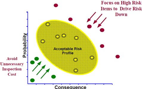
Fig. 1 illustrates the main concept of RBI is managing risk and developing the required action based on the equipment risk profile. The risk model is used to calculated the risk associated with all equipment, and by defining the risk tolerance resources and attention can be concentrated on those equipment items that present the highest potential losses or consequences. The challenge in doing this lies with the difficulty in establishing the risk tolerance/risk target to segregate high and low risk equipment, and consequently define the equipment that may need further maintenance and inspection and other equipment that need less inspection or may eliminate unnecessary inspections. Assigning the inspection and maintenance resources in proportional to equipment adherent operational risk will result in optimizing resources without compromising the equipment mechanical integrity. If the equipment operational risk was not estimated correctly and/or an adequate risk target was not established, the results will be either, overlooking some critical equipment, assigning maintenance and inspection resources to the wrong equipment or give a false feeling of safety which leads to relaxing important inspection and maintenance activities. These misleading results of RBI assessment can jeopardize the plant integrity and fail in achieving the main objective of RBI assessment.
Level 1 and 2 regimes provide a distinct equation for liquid and vapor release rates; and hence the release phase needs to be determined first to apply the adequate release rate equation. Level 2 consequence analysis models use two-phase releases and distinguish between the amount of the theoretical release rate that releases liquid to the atmosphere as vapor or as an aerosol (vapor with entrained liquid) in the form of a jet and the amount of the release that drops to the ground as liquid to form a pool.
For level 2 the actual composition of the fluid, including mixtures, should be used in the analysis; therefore, fluid property solvers are needed to calculate fluid physical properties more accurately. The fluid solver provides the ability to perform flash calculations for better determination of the release phase of the fluid and to account for two-phase releases. The fluid property calculations in Level 2 are focused on flash calculations that are applicable to liquid or two-phase releases. The offshore production platform included in this assessment produces gas (i.e., 70 % methane, 11-12 % nitrogen and other hydrocarbons) and so the flash calculations are not applicable. The DIPPR database is used to determine the fluid properties and the isentropic flash calculations are undertaken to calculate the properties at release conditions. Level 2 analysis requires a fluid property package to isentropically flash (isenthalpic is acceptable) the stored fluid from its normal operating conditions to atmospheric conditions. In addition, the effects of flashing on the fluid temperature as well as the phase of the fluid at atmospheric conditions should be evaluated. Liquid entrainment in the jet release as well as rainout effects could be evaluated to get a more representative evaluation of the release consequences.
The probability of ignition (POI) model adapted in level 2 consequence methodology is based on a study by Cox [15] that presented a simple generic POI distribution that correlates the POI with the mass release rate. This model is developed based on ignition incidents of major blowouts from experience basically during the period of 1970s and 1980s. The more recent blowout incidents analysis concluded lower POIs. Large releases at process facilities may have less POI due to the presence of fewer of ignition sources and lower inventories available for release. This model does not consider the key differences between onshore and offshore environments that includes the confined layout of most offshore installations as opposed to the relatively open nature of many onshore facilities. [16] UKOOA reviewed all available ignition probability models such as Cox, Lee and Ang, and found them to have relatively weak foundations whereas there are anchored to a few actual data points based on blowout data that is now out of date.
[14] demonstrated how the release type is critical in the API methodology [12, 13] whereas the calculated consequences differ greatly depending on the type of release, i.e., continuous or instantaneous. This results in quite different total risk, and so a different course of action is needed to manage that risk. Despite the paramount criticality of defining the flow type, there is no precise or objective criteria for defining the release type. The methodology [12, 13] does not consider the potential area of exposure (i.e., the area of the offshore platform was exposed to the consequences, for example in the case of leak on cellar deck, potential exposure area could be higher than the total area of the platform.
To evaluate the reliability and subjectivity of the API methodology risk results, this paper presents evaluations of actual risk assessment conducted on topside equipment of an offshore platform using the two consequence models (i.e., level 1 & 2), furthermore, sensitivity analysis was performed for the PoF model and the final risk results were critically discussed. The case study presented in this paper demonstrates how the subjectivity in the risk models can lead to completely different results, consequently, courses of action. The PoF sensitivity analysis illustrates the impact of contributing factors to the PoF model to quantify the reliability and subjectivity in the failure probabilities. A comparison between both API consequence modelling methodologies (i.e., CoF level 1 and 2) was performed to manifest the reliability of risk results. This critical discussion has a paramount importance to the maintenance and operations personnel who adapt these RBI methodologies to determine the inspection and maintenance plans. The decision-maker should be attentive to the subjectivity and reliability of the resulting risk to establish an adequate risk target that can achieve the ultimate goal of RBI by determining the cost-effective inspection and maintenance plan without compromising the plant safety, integrity or reliability.
2. Description of adapted risk model
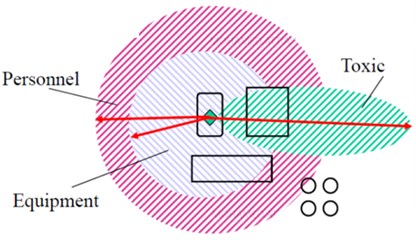
Risk is estimated in for different possible consequences of failures i.e., equipment damage, personnel injury and toxic injury. The impact of each consequence is presented in form of affected area as shown in Fig. 2.
Fig. 2Consequence of failure affected areas
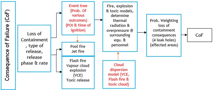
The PoF model as outline in Fig. 3, is based on the estimating the fraction of wall loss and limit sate function along with inspection history to determine the reliability index then damage factor. API 581 introduces to models to calculate CoF. [14] Level 1 CoF model is based on a pre-developed set of lookup tables for specific fluids in refinery and petrochemical plants, while Level 2 CoF model is based on rigorous calculations that can address the exact stream composition and precisely calculate the consequence area for several flammable and toxic event outcomes (i.e., event tresses). Therefore, fluid property solvers are needed to calculate fluid physical properties more accurately. The fluid solver provides the ability to perform flash calculations for better determination of the release phase of the fluid and to account for two-phase releases. The fluid property calculations in Level 2 are focused on flash calculations that are applicable to liquid- and two-phase releases. Fig. 4 provide outlines for level 2 consequence model.
The PoF model is based on the parameter that estimates the fraction of metal loss and certain time of the equipment operational lifetime. The factor is used along with the past inspection effectiveness to determine a damage factor (DF). The basic function of the DF is to statistically evaluate the amount of damage that may be present as a function of time in service and the effectiveness of an inspection activity. Damage factors with a value greater than 1.0 will increase the probability of failure, and those with a value less than 1.0 will decrease it. The total damage factor is an accumulation of all applicable damage mechanisms or combination of damage mechanisms. The adjustment factors are applied to the generic failure frequencies to reflect departures from the industry data to account for damage mechanisms specific to the components operating environment and to account for reliability management practices within a plant. The damage factor is applied on a component and damage mechanism specific basis.
Fig. 3Overview of the PoF model
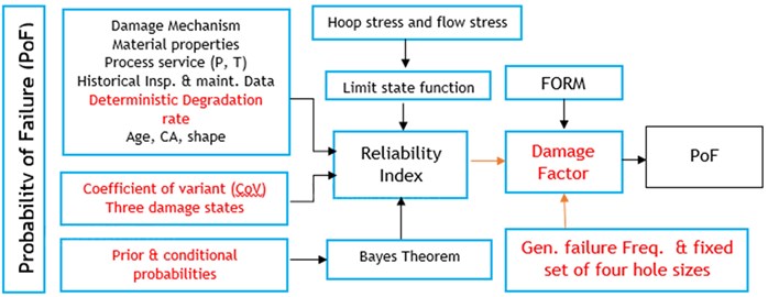
Fig. 4Overview of the CoF level 2 procedure
The PoF is calculated using structural reliability for load and material strength (flow stress) based on result in plastic collapse failure. Flow stress is the minimum stress required to sustain plastic deformation of a pressure-containing envelope to failure. The structural reliability model is integrated with a Bayes’ theorem to allow credit for the number and type of inspections performed on the PoF and total risk. The uncertainty in the rate of metal loss (i.e., corrosion rate) is quantified by the number and effectiveness of past inspections. The confidence level in the corrosion rate increases with more in-service inspections and the effectiveness of these inspections in quantifying the actual condition of the equipment. The DF is updated based on the confidence in the corrosion rate provided by using Bayes Theorem.
The methodology assigns discreet random variable to the corrosion rate. The ability to state the corrosion rate precisely is limited because of the equipment complexity, process and metallurgical variations, inaccessibility for inspection, and limitation of inspection technologies. Therefore, to account for the uncertainty in metal loss (corrosion rate), three damage states were used in the methodology:
Damage state 1 – The real corrosion rate is equivalent to the measured corrosion rate; Damage state 2 – The real corrosion rate is double the measured corrosion rate; Damage state 3 – The real corrosion rate is four-times the measured corrosion rate. As metal loss continues over time, the DF increases until the risk target is reached. Therefore, some inspection would be performed.
The coefficient of variances (COV) was assigned for three key measurements affecting POF, as follows: COV for thickness, () ; to quantify the uncertainty in inspection measurement accuracy, COV for pressure, () ; to presents uncertainty is accuracy of pressure measurements, and the COV for flow stress, () ; uncertainty of actual TS and YS properties of equipment materials of construction.
Loss of containment of hazardous fluids from pressurized processing equipment may result in damage to surrounding equipment and serious injury to personnel. The CoF methodology quantifies the impact areas from event outcomes such as pool fires, flash fires, fireballs, jet fires, and vapor cloud explosions, based on the effects of thermal radiation and overpressure on surrounding equipment and personnel. The API model outlines two methods of analysis to calculate the CoF; A level 1 CoF approach that is based on a pre-developed set of lookup tables for common fluids in refinery and petrochemical plant. As we can see on the event tree, level 1 does not address two phase flow. Moreover, the POI and probabilities of other release events used to develop the lookup tables are constants, i.e., independent of the release rates. Level 2 CoF analysis that is based on rigorous calculations that can address the exact stream composition to calculate the consequence area for serval flammable and toxic event outcomes. Main part of level 2 calculation is dispersion modelling; however, the API methodology do not provide any specific dispersion model or specify certain requirements need to be addressed in the dispersion modelling. [17] introduced gas dispersion model can be used in the consequence calculations, however, that model is adequate only for light hydrocarbon gases (e.g., C1-C2).
3. Risk assessment/case study
The case study was performed using these two different CoF procedures to point out the gaps and shortcomings of each procedure. the adapted dispersion model in level 2 calculation was based on SLAB model that can treats denser-than-air releases. The case study performed on topsides static mechanical pressure systems at offshore platform, whereas, the pressure system boundaries are the Christmas tree wing valve through to the export pipeline topsides emergency shutdown (ESD) valve. This involves the following types of components: Piping systems comprising straight pipe, bends, elbows, tees, fittings, reducers, pressure vessels and atmospheric tanks, scraper launchers and receivers, valves, etc.
3.1. Probability of failure
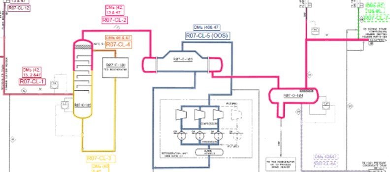
Fourteen corrosion loops were identified for the selected equipment and piping systems on the platform. Corrosion loops are defined on the basis of process/fluid composition and material of construction, and active corrosion or degradation mechanisms. The applicable damage mechanisms have also been marked and numbered on process flow diagrams (PFD’s). wet H2S damage (i.e., HIC, SSC), CO2 corrosion, sour water corrosion, and external atmospheric corrosion are the main damage mechanisms applicable in this assessment. Fig. 5 shows an example of the corrosion loops drawing.
The damage factor is estimated based on the strength ratio, whereas two equations are given for calculation of the strength ratio [2]:
where : operating pressure, : component diameter, : flow stress, : weld joint efficiency, : allowable stress, : minimum required thickness, : minimum structural thickness and : minimum measured thickness.
The flow stress is the average of the yield stress and the tensile strength of the material, which would be likely to be approximately twice the allowable stress for a modern vessel designed to ASME Division 1/2, or BS EN 13445. Therefore, with no thinning, the value of would be approximately 0.5, and the damage factor would be negligible. With a thinning to half the minimum thickness, the SR value would increase to 1, with DF = 3200. The calculations do not consider the extent of the thinning, so highly localized thinning would be treated the same as general corrosion.
Fig. 5Sample of corrosion loops
Sensitivity analysis was performed to evaluate the impact of on the external damage factor, all other input parameters in thinning calculations such as (Pressure Coefficient of Variance) and (Flow Stress Coefficient of Variance) are fixed moreover, the corrosion rate was assumed constant over the design life time. Fig. 6 shows that the impact of , increases over the lifetime.
Fig. 6Influence of COV∆t on external DF
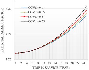
Fig. 7External DF sensitivity analysis to COV∆t with progressive external corrosion rate

External corrosion DF:
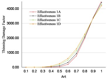
Assuming the corrosion rate will be constant over the design lifetime, even though the operating conditions are not changed, may not be plausible. Therefore, this sensitivity analysis is reconstructed to account for different corrosion rates over the life cycle. Fig. 7 illustrates the correlation between the damage factor and factor that accounts for time in service and the corrosion rate.
The analysis demonstrates how the calculated damage factor is very sensitive to the value of , especially with aging equipment experiencing a sever corrosion rate. For example, at = 0.5 the calculated DF rise up 2.9 times, i.e., from 150 at 0.1, into 436 at 0.2.
Internal corrosion DF:
Fig. 8 shows how the calculated DF is very sensitive to the value of especially with progression in time and corrosion rate. For example, at 0.3 when using = 0.1 the resulting DF is 0.14, while the resulting DF is 14.07 when 0.2, i.e., the DF is raised more than 100 times. This analysis shows how the calculation of DF is very sensitive to the value of .
Fig. 8Thinning damage factor sensitivity to COV∆t
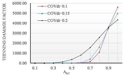
Fig. 9Thinning damage factor sensitivity to COVp
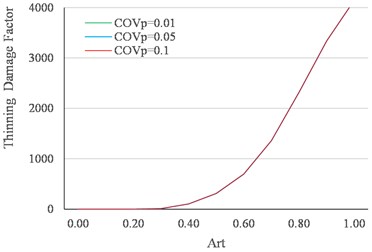
The calculation of DF was found not sensitive to the or as shown in Figs. 9 and 10.
Fig. 10Thinning damage factor sensitivity to COVsf
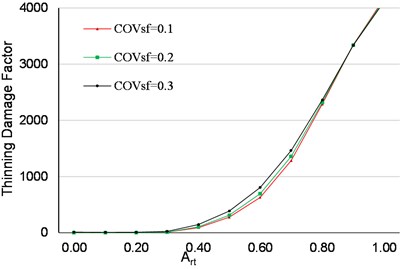
Fig. 11Effect of confidence level with constant internal corrosion rate
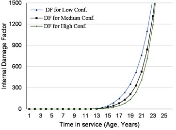
One of the key factors in calculating the PoF is the prior probability, which depends on the confidence level of inspection data (corrosion rate) as show in Table 1. There is no scientific basis for these prior properties; they have been established based on individuals’ judgment. Therefore, sensitivity analysis was performed to evaluate the impact of this assumption on the calculation of damage factor. Fig. 11 shows that the sensitivity of internal damage factor to the data confidence is significantly increases with the age of the piping after 10 years of service. This impact makes the PoF calculation quite subjective especially with equipment aging.
Table 1Prior probability for thinning corrosion rate
Damage state | Low confidence data | Medium confidence data | High confidence data |
0.5 | 0.7 | 0.8 | |
0.3 | 0.2 | 0.15 | |
0.2 | 0.1 | 0.05 |
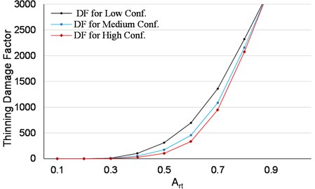
The above sensitivity analysis assumed the corrosion rate is constant over the design lifetime. To account for the regression corrosion rate, the damage factor presented Vs. the parameter as given in Fig. 12. This analysis highlights the discrepancy in calculating the damage factor, for example at 0.3 and with low confidence the DF is 3.7 times (DF = 10.53) the calculated DF at high confidence (DF = 2.91), at 0.6 with low confidence level the DF = 695 and would be 334 if the confidence level set to high i.e., the difference is more than double. These results demonstrate how the calculated DF can be inconsistent, subjective and very sensitive to the user’s inputs.
Fig. 12Effect of confidence level with regression internal corrosion rate
Reduction in uncertainty in the damage state of a component is a function of the effectiveness of the inspection to identify the type and quantify the extent of damage. Inspection plans are designed to detect and quantify the specific types of damage expected such as local or general thinning, cracking and other types of damage. An inspection technique that is appropriate for general thinning will not be effective in detecting and quantifying damage due to local thinning or cracking. Therefore, the inspection effectiveness is a function of the inspection method and extent of coverage used for detecting the type of damage expected. Figs. 13 and 14 illustrate the impact of inspection effectiveness category from A to D on the calculated damage factor. Sensitivity analysis is performed for different inspection effectiveness category with the same number of inspections. Where the inspection effectiveness is changing from A (highly effective) to D (poorly effective).
Fig. 13Sensitivity to inspection effectiveness (no. of inspections = 1) with a constant corrosion rate
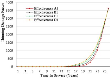
The effect of inspection effectiveness rises with time and higher corrosion rate for example at 0.5 the calculated DF = 34 when “A” inspection effectiveness is conducted. DF leaps to 185 when inspection effectiveness is set to “C.” This represent more than around 5.5 time increases in the DF and PoF. Both of inspection effectiveness category and model the uncertainty in inspection data. The sensitivity analysis demonstrated how the DF calculation is very sensitive to the values of these two factors. addressing the uncertainty twice results in exaggerating the calculated DF & PoF.
Fig. 14Sensitivity to inspection effectiveness (no. of inspections =1)
Total thinning DF:
In the case study presented in this paper, the potential damage mechanisms cause general corrosion; therefore, the damage is likely to occur at the same location hence, the total DF is given as:
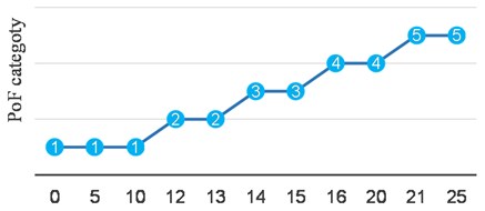
Fig. 15 represents the calculated damage factors including internal, external and total damage factors with time in service. Figure 16 illustrates the probability of failure category over the design lifetime.
Fig. 15Damage factors over the design lifetime
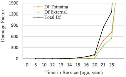
Fig. 16PoF category over the design lifetime
The PoF model does not address the statistical distribution of corrosion rates (e.g., normal, lognormal, Weibull, etc.), but use only COV and inspection effectiveness categories which, make the results more subjective and cast doubt on the reliability of the PoF calculations consequently, the resulted inspection plan. Especially for inspection plans that are driven by the PoF. Furthermore, the background of the 1.56 E -04 constant that is used to convert the PoF into DF has never been documented in any of the editions of API RP 581. The authors understanding of this factor is that it was the failure frequency in units of failures/year for fixed equipment based on a review of industry failure data. This, in essence, was the initial generic failure frequency (GFF) used by the API. The initial GFF was broken into four holes as follows; leak frequency per hole size: 0.25” hole – 4 E-5, 1.00” hole – 1E-4, 4.0” hole – 1 E-5, rupture – 6 E-6:
Gff = 4 E-5 + 1 E-4 + 1 E-5 + 6 E-6 = 1.56 E-4 frequency/year.
By dividing the PoF by the GFF, this will not convert the PoF to a dimensionless parameter (i.e., DF). Dividing the dimensionless PoF (0 to 1) by a frequency (failures per year) results in a DF with units in years/failure, not a dimensionless factor as stated in API RP 581.
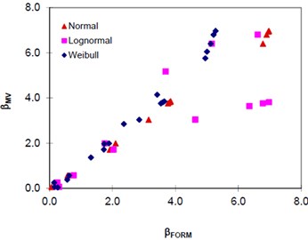
The mean-value first-order reliability method (MVFORM), which is adapted in the DF calculation, [18] This method uses the first order moment of limit state function at mean value point of random variables to obtain the mean value
and standard deviation of limit state function. Therefore, DF calculations use mean value and standard deviation of the material yield strength and load. Even though, MVFORM is simplest and easiest method to approximate the mean value and standard deviation of limit state function, does not give the best results [19] compared to the reliability indices calculated by MVFORM with FORM using three different distribution types (normal, Weibull, and lognormal) as illustrated in Fig. 17. The results showed that reliability indices of 4 are comparable for all three distributions; however, the results diverge when 4. In other words, MVFORM is less accurate when estimating the PoF at high reliability index, (id very low probability of failure).
Fig. 17Comparison of β calculated using FORM, βFORM and MVFORM, βMV
3.2. Consequence of failure
There are two steps for evaluating the consequences:
a) Scenario Selection: The scenarios to be considered for the failure of and equipment or circuit should be identified considering the different leak failure modes.
b) Scenario Modeling: For each possible failure scenario the following should be applied:
1) Estimate the available mass.
2) Estimate the discharge rate.
3) Evaluate dispersion models.
4) Assessment of impacts from fire, explosion and toxicity.
API Level 1 CoF model provides a predefined list of common fluids, lookup tables and charts. For the Level 1 analysis, a series of consequence analyses were performed to generate consequence areas as a function of the reference fluid and release magnitude. Probabilities of ignition, probabilities of delayed ignition, and other probabilities in the Level 1 event tree were selected based on expert opinion for each of the reference fluids and release types (i.e., continuous or instantaneous). These probabilities were constant and independent of release rate or mass. Level 2 offers a rigorous calculation for consequences when data are not provided for the fluids mentioned in level 1, or when assumptions made in level 1 are not valid.
This case study was performed for topside static equipment at offshore platforms to qualify the discrepancy in calculating the CoF using level 1 and 2 methodologies. The offshore facility included in this assessment is gas compression plant. The main process is producing compressed gas that is shipped from offshore to a gas plant. The feed gas comes from the other offshore producing platforms, in addition, there are supporting or utility process which are related to the dew point system and process cooling water requirement. Gas compression plant consists of three decks, these are the main deck, which counts for an area of approximately 4716.4 m2 and a cellar deck, which counts for an area of 4597.42 m2. Thus, the total area for both decks is around 9313.8 m2. For the third deck, it is a spider deck, which is only a walkway. The platform was built in 1992 and it can produce up to an operating capacity of 580 MMSCFD and design capacity of 954 MMSCFD. The sour gas processed is approximately 15000 ppm of H2S concentration. The process area consists of the three processing trains, two of which are in operation and other one is a standby. The study covered all of the three trains.
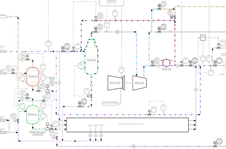
Inventory groups were developed to determine the mass of fluid that could realistically be released in the event of a leak or rupture from pressure boundary components. When a component or piece of equipment is evaluated, its inventory is combined with inventory from other attached equipment within its inventory group that can realistically contribute fluid mass to the component that is leaking. The inventory groups are determined based on an assessment and review with operations personnel with consideration given to the presence of control valves that can be remotely activated to isolate the plant in case of an emergency situation. Twenty-seven inventory groups were identified. These have been highlighted and color coded on PFDs. Fig. 18 shows a sample of the inventory group drawing.
Fig. 18Sample of inventory groups
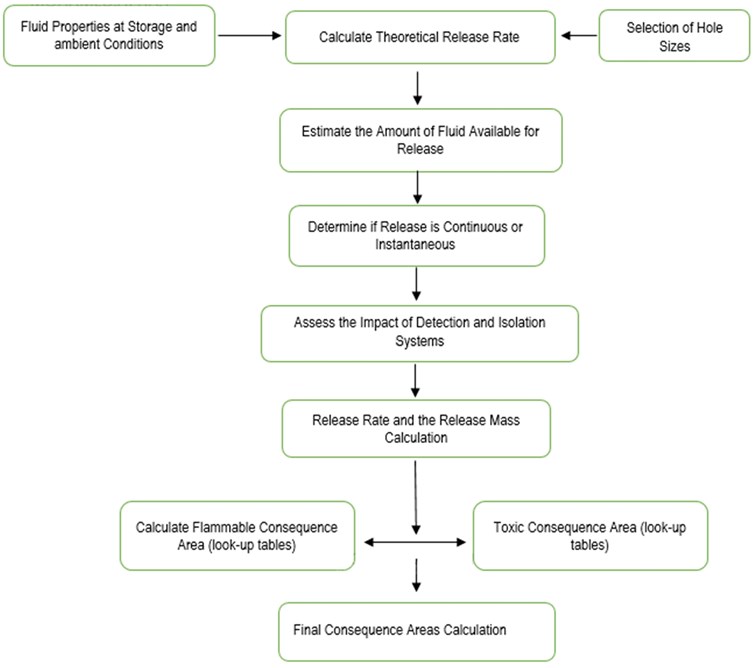
The consequences of releasing a hazardous fluid are estimated in eight distinct steps:
1) Determining representative fluid and its properties.
2) Selecting a set of hole sizes, to find the possible range of consequences in the risk calculation.
3) Estimating the total amount of fluid available for release.
4) Estimating the potential release rate defining the type of release, to determine the method used for modeling the dispersion and consequence.
5) Selecting the final phase of the fluid, i.e., a liquid or a gas.
6) Evaluating the effect of post-leak response.
7) Determining the area potentially affected by the release.
Fig. 19 illustrates the outline of calculating consequence areas.
Fig. 19Flowchart for calculating level 1 consequence area
3.3. Risk analysis
Presenting the risk results in a matrix is an effective way of showing the distribution of risks for components in a process unit without using numerical values. Therefore, a risk matrix is typically used in risk assessment studies; it allows the user to present the total risk of every equipment and determines the required risk reduction measures in a manner that is proportional to the level of risk. In the risk matrix, PoF and CoF categories are arranged so that the highest risk components are toward the upper right-hand corner. There is a wide spectrum of risk matrix configuration that are being used; however, the more cells we have in the matrix, the higher resolution in defining the risk precisely. For this case stud a 7×7 matrix was used, Fig. 20 shows the risk matrix with the four distinguished risk categories. A comparison between the risk distribution resulted from level 1 and 2 is presented in Fig. 21. For example, the number of equipment lay at medium-high risk is only 34 per level 1 assessment results while it is 64 equipment based on level 2 assessment.
Table 2 summarizes the variance in the calculated risk and the risk distribution. For example, using level 2 CoF resulted in having double the number of equipment lay in the medium high-risk categories using level 1 CoF. The variance in the total risk of all equipment included in the assessment is 59 % that means the calculated risk using CoF level 2 is more than double the calculated risk using level 1. This significant variance in the calculated risk can dramatically affect developing the action plans. The optimum plan should be developed to reduce the risk to an acceptable threshold. In fact, this significant variation in the results can hinder the operator to define what would be the reasonable and cost-effective risk tolerance that should be used to develop inspection and maintenance plans.
Fig. 20Risk matrix for a level 2 assessment
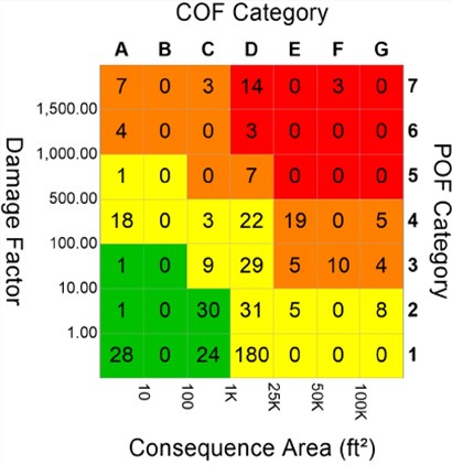
Fig. 21Comparison of risk distributions
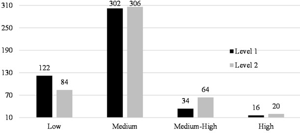
Table 2Summary of calculated risk variance
CoF | Total risk (ft2/yr) | Average risk (ft2/yr) | Avg. CoF (ft2) | Low | Medium | Medium-High | High |
Level 1 | 42241.15 | 89.12 | 5855.14 | 122 | 302 | 34 | 16 |
Level 2 | 67279.95 | 141.94 | 14975.01 | 84 | 306 | 64 | 20 |
Variance (%) | 59 | 59 | 55 | 31 | 1.32 | 88 | 25 |
4. Results discussion
The sensitivity analysis demonstrated the significant impact of the prior probabilities on the calculated DF. These values are assigned based on judgment without a scientific basis, which makes the PoF calculations very subjective. Furthermore, the uncertainty in inspection data is addressed twice in the PoF model by different factors, i.e., inspection effectiveness category and , that duplication affects the results. The sensitivity analysis demonstrated how the DF calculation is very sensitive to the values of these two factors, which makes the risk results inconsistent and subjective. This duplication in addressing the uncertainty exaggerates the calculated PoF.
The design features of an offshore platform such as the influence of having fire/blast walls are not addressed in calculating the consequence area. For example, if the jet fire cannot be maintained for the duration for which the fire wall is rated, then the consequence area should be limited to the area within the firewalls. The methodology does not consider the potential area of exposure (i.e., the area of the offshore platform exposed to the consequences, for example in the case of leak on cellar deck, potential exposure area could be higher than the total area of the platform. For example, in the case of a scraper launcher, the consequence area is calculated using level I methodology was more than 1500 m2. The variance in the calculated risk was more than 59 % between level 1 and level 2 consequence methodologies.
5. Conclusions
The sensitivity analysis performed on actual top-side static equipment at offshore platform demonstrated the subjected in the PoF calculations and how the results are very sensitive to the assumption make by the analysist who perform the assessment. Moreover, the results of CoF results are vary depend on which consequence model is used, i.e., level 1 or level 2.
As demonstrated in this paper the key task in determining the outcome of RBI assessment, is the criterion of segregating equipment items that have acceptable and unacceptable risk. This is the main gate to determine whether a certain course of action needs to be developed to manage this risk. The end-user needs to be vigilant to the accuracy and precision of the risk model used to determine the adherent operational risk to the equipment items. Hence, a genuine risk target can be established to determine which equipment needs a certain course of action to manage risk, and other equipment that is needed to eliminate inspection and maintenance activities to avoid unnecessary inspections/maintenance. Determining adequate risk target will lead to developing the most cost-effective inspection and maintenance plans, without compromising the asset integrity. Therefore, the end-users need to be vigilant to this significance difference in the calculated risk resulted from different consequence and probabilities modellings while establishing the risk tolerance. Otherwise, the significance in the calculated risk may result in misleading inspection and maintenance plans that either overlook critical equipment or spend unnecessary resources on performing inspection and/or maintenance for unnecessary activities that do not contribute effectively to managing the plant’s operational risk. In other word, there is no single adequate risk tolerance/target which can be utilized for all different risk models, moreover, the configuration of risk matrix should be determined according to the utilized risk model and established risk target.
The work presented in this paper revealed the need to develop more objective risk model especially for offshore platforms to address the unique features of consequence modelling.
References
-
F. Khan, R. Yarveisy, and R. Abbassi, “Risk-based pipeline integrity management: A road map for the resilient pipelines,” Journal of Pipeline Science and Engineering, Vol. 1, No. 1, pp. 74–87, Mar. 2021, https://doi.org/10.1016/j.jpse.2021.02.001
-
R. Mohamed, C. R. Che Hassan, and M. D. Hamid, “Implementing risk-based inspection approach: Is it beneficial for pressure equipment in Malaysia industries?” in Process Safety Progress, Vol. 37, No. 2, pp. 194–204, Jun. 2018, https://doi.org/10.1002/prs.11903
-
Deighton Michael, Facility Integrity Management: Effective Principles and Practices for the Oil, Gas and Petrochemical Industries. Oxford: Elsevier Science & Technology, 2016.
-
U. R. Bharadwaj, V. V. Silberschmidt, and J. B. Wintle, “A risk based approach to asset integrity management,” Journal of Quality in Maintenance Engineering, Vol. 18, No. 4, pp. 417–431, Oct. 2012, https://doi.org/10.1108/13552511211281570
-
K. Bhatia, F. Khan, H. Patel, and R. Abbassi, “Dynamic risk-based inspection methodology,” Journal of Loss Prevention in the Process Industries, Vol. 62, p. 103974, Nov. 2019, https://doi.org/10.1016/j.jlp.2019.103974
-
R. Com, “Risk-Based Inspection (RBI) Program Implementation Case History,” Inspectioneering Journal, 2017.
-
“Base Resource Document on Risk-Based Inspection for API Committee on Refinery Equipment,” American Petroleum Institute, 1996.
-
“Risk-Based Inspection Technology,” 3rd. Edition, API Recommended Practice 581, May 2000.
-
“PCC-3 Inspection Planning Using Risk-Based Methods,” American Society of Mechanical Engineers, 2007.
-
Risk Based Inspection – A Guide to Effective Use of the RBI Process. EEMUA Publication, 2006.
-
“Recommended Practice for Risk-Based Inspection,” American Petroleum Institute, 2016.
-
“Risk-Based Inspection Technology,” American Petroleum Institute, 2nd. Edition, API Recommended Practice 581, 2008.
-
“Risk-based Inspection Methodology,” American Petroleum Institute, 2016.
-
M. Attia and J. K. Sinha, “Reliability of quantitative risk analysis through an industrial case study,” Journal of Quality in Maintenance Engineering, Vol. ahead-of-print, No. ahead-of-print, Nov. 2021, https://doi.org/10.1108/jqme-03-2021-0022
-
A. W. Cox, F. P. Lees, and Ang M. L., “Classification of Hazardous Locations,” Institution of Chemical Engineers, 1991.
-
“IP Research Report: Ignition Probability Review, Model development and Look-Up Correlations,” Energy Institute, London, 2006.
-
M. Attia and J. Sinha, “Improved quantitative risk model for integrity management of liquefied petroleum gas storage tanks: Mathematical basis, and case study,” Process Safety Progress, Vol. 40, No. 3, pp. 63–78, Sep. 2021, https://doi.org/10.1002/prs.12217
-
C. A. Cornell, “First-order uncertainty analysis of soil deformation and stability,” in First International Conference on Application of Probability and Statistics in Soil and Structural Engineering, pp. 129–144, 1972.
-
A. Tallin, and M. Conley, “Assessing inspection results using Bayes’,” in 3rd International Conference and Exhibition on Improving Reliability in Petroleum Refineries and Chemical Plants, 1994.
Cited by
About this article

