Development of an underwater robotic arm using multibody dynamics approach

1. Introduction

Ships or vessels that are submerged partially or completely underwater are constantly in contact with various living organisms that are inhabited in these bodies [1]. These organisms tend to get contaminated the surfaces of submerged bodies resulting in degrading of the hull and even causing significant amounts of drag opposing the motion of the vessel.

Throughout the history, engineers have incorporated various techniques to clean the surface, by manual and automated methods. These cleaning methods are mainly divided as, Dry-dock cleaning and underwater cleaning [1]. Underwater cleaning was used to be done by professional divers going to the bottom of the vessel and manually cleaning the hull which was however mostly ineffective and unsafe. More recent advancements in technology enabled complete remotely operated cleaning of the hull surface of the ships. When it comes to operations such as welding and painting the accuracy of the movement is very important which is very difficult to obtain due to both inertia and hydrodynamic forces. The scope of this investigation is to develop a 6 DOF underwater robotic manipulator which will move a desired cleaning system (Laser Cleaning or pressure cleaning) around a 3D space providing the necessary accuracy.

When designing a manipulator, DH parameters is an important data set that is required to analyze the kinematics of the model [2]. However, [3] shows a method that can be used to find the kinematic solutions of a model of up to 6 DOF by using 7 basic parameters which can be easily derived from the manipulator dimensions. This study has used the above method to solve the kinematic solutions to the model. In addition to that, for underwater systems, fluid dynamic and buoyancy forces must be considered simultaneously when controlling the manipulator [4]. The positioning of the end effector while the base is connected to a floating body has a strong inertia and hydrodynamic coupling. The controller should take all these into consideration simultaneously for precise operation [5]. In this study a virtual model has been built in multibody dynamics environment where all these physical phenomena can be connected together such that the actual control strategy can be fully developed, and necessary gains can be selected. Furthermore, authors are expected to extend this work by incorporating the component flexibility and tribological aspects of the contact conjunctions of the robot arms. Such an extension will only be possible in the multibody dynamics environment which uses the Lagrange methods to formulate the equations [6]. Through this the accuracy of the end effecter will further be improved.

Fig. 17 Parameters used for solving kinematics [3]

a) Side view

b) Back view

2. Mathematical model of the 6DOF manipulator

The initial simulations for the robotic manipulator designs were done using MATLAB Simulink multibody-dynamics environment by importing the CAD models built from solid works. However, the models were later transferred to ADAMS software since it was simpler to visualize the mechanics of the model. Then, for the implementation of the control system, MATLAB-ADAMS co-simulation was used.

After the open loop kinematics analysis, it was later decided that the use of a 6 DOF manipulator with wrist joints would be much beneficial due to its ability to change the orientation of the end effector frame [2]. The three degrees of freedom manipulator lacked the ability to change the orientation of the end-effector frame. This issue was solved by upgrading to a higher degree of freedom system.

The definition of above parameters in Table 1. that are used in solving the inverse kinematic solutions for the 6 revolute joints representing the 6-DOF can be found in the Fig. 1. 7 Parameters used for solving kinematics.

The fluid dynamic forces were introduced to the manipulator and the inverse kinematics for the 6-DOF system was developed after carefully reviewing the literature of the kinematic analysis for the manipulator[3].

The fluid dynamic forces considered in this study are the buoyancy forces and the profile drag forces that are acting on the model. The formula for the buoyancy forces acting on the centre of buoyancy of each link can be expressed as shown below:

where ${\rho }_{fluid}$ is the density of the fluid, $V_{eff}$ is the effective volume of fluid that is displaced due to the body and g is the gravitational acceleration.

The profile drag component of the fluid dynamic forces can be expressed as a function of the square of the velocity $\left(v^2\right)$ of the body, the drag coefficient $C_d$, the density ${\rho }_{fluid}$of the fluid and the effective area that $A$. The formula for the profile drag force acting on the centroid of the links due to the motion of the manipulator can be expressed as shown below:

Fig. 2a) Rotated view and b) Side view of the robotic manipulator [3]

a) Rotated view of manipulator

b) Side view of manipulator

The kinematic solutions of the of the system were implemented based on the method introduced in [3] by using the dimensional parameters of the designed robotic manipulator given in Table 1. The expressions for the forward kinematics of the model can be derived as:

where, $c_{x1}$, $c_{y1}$, $c_{z1}$ are the coordinates of the tip of the end effector from the side view shown in Fig. 2(b) and $c_{x0}$, $c_{y0}$, $c_{z0}$ are the coordinates of the final position of the end effector relative to the given joint angles.

The first two of the multiple solutions related to the first three joint angles can be derived using the inverse kinematic equations which can be expressed as shown below:

where, ${\theta }_1$, ${\theta }_2$, ${\theta }_3$ are the first two solutions of the positioning joints, $n_{x1}$ is the distance between $G_2$ axis and $C$ and:

3. Results and discussion

Th results given in this paper are based on the 6-DOF manipulator model and the square shaped desired trajectory 1-4 given in Fig. 3.

Fig. 3Labelled diagram of the 6-DOF manipulator Adams model with the trajectory

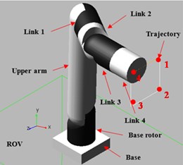
After the implementation of the inverse kinematics of the manipulator and the control strategy using PID controllers, it was identified that the velocity profile of the joint motions had to be controlled to achieve a smooth motion with minimum amount of peaking of the joint torques. For this, a trajectory with polynomial velocity profile was developed using Robotic Operating Systems (ROS) toolbox in Matlab Simulink. The resulting polynomial velocity profiles are shown in Fig. 4 and Fig. 5.

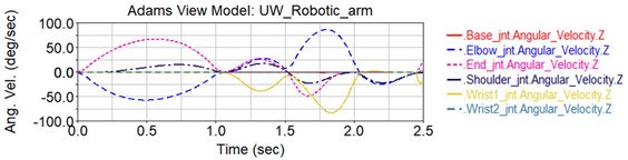
Fig. 4Polynomial velocity trajectory of the Base joint

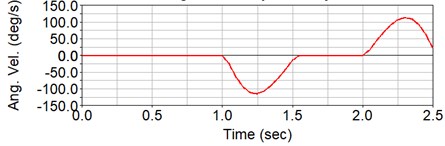
Fig. 5Angular velocities around the z axis of the six individual joints

In order to establish the hydrodynamic environment, the buoyancy forces and the drag forces were introduced to the multibody model using the Adams software.

The buoyancy forces acting on each link of the manipulator arm are always constant since the manipulator is fully submerged inside the water body during the operation. Therefore, the buoyancy force acting on each link can be calculated using the effective volume of the link $V_{eff}$ and Eq. (1).

The drag forces applied on the upper arm around the global $y$ axis can be graphically shown as below in Fig. 6.

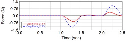
The graphical representation of the drag force acting on the links 1 and 2 around the global $z$ axis and the global $y$ axis due to the motion can be shown as in Fig. 7 and Fig. 8.

Fig. 6The drag force acting on the upper arm due to the motion

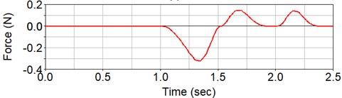
Fig. 7Drag force acting on the Links 1, 2 around the global z axis

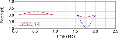
Fig. 8Drag force acting on the Links 1, 2 around the global y axis

When the manipulator is in motion, there will be forces induced as a result of the inertial forces and the hydrodynamic forces available in the system. The resultant of these forces will act on the ROV at the base of the manipulator where it is mounted to the ROV. They also create a torque around the global $y$ axis of the manipulator. The resultant torque will act on the ROV at the centre of mass.

The vertical force that will be created at the base of the 6-DOF manipulator can be shown as in Fig. 9 and the torque that will be created at the centre of mass of the ROV can be shown as in Fig. 10.

Fig. 9The total vertical force acting on the ROV due to the inertial forces and the hydrodynamic forces

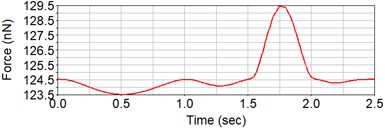
Fig. 10The total torque acting on the ROV due to the inertial forces and the hydrodynamic forces

To achieve optimum control of the manipulator, the PID controllers of each individual 6 degrees of freedom were tuned separately [7].

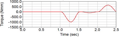
After tuning the PIDs, the resulting torque at the base joint was observed as shown below in Fig. 11.

Fig. 11Torque needed for the motion at the base joint

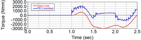
Fig. 12Deviation of actual end-effector x coordinate from the desired y-z plane

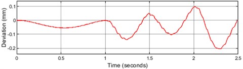
The trajectory given is on a on the $z$-$y$ plane. This makes the displacement in the $x$ direction constant. The deviation of the end-effector $x$-coordinate with reference to the desired $x$-coordinate after the tuning of the PIDs is shown by Fig. 12.

4. Conclusions

The main objective of the project was to develop and implement the control strategy of a robotic manipulator that is supposed to be used in the shipping industry for maintenance purposes. The initial design of the robotic manipulator yielded certain limitations. These limitations were overcome by improving the initial design of 3 degrees of freedom to a 6 degree of freedom system. The trajectory planning was done to make the end-effector follow the path that represent the coordinates that were input to the model, and the final results of the joint motions were analyzed. The forces and torques applied at each joint to achieve the desired motion were analyzed and controlled using Feedback PID Control. Further improvements can be done to optimize the control of the manipulator to improve sensitivity of the trajectory of the end effector.

References

-
C. Song and W. Cui, “Review of underwater ship hull cleaning technologies,” Journal of Marine Science and Application, Vol. 19, No. 3, pp. 415–429, Sep. 2020, https://doi.org/10.1007/s11804-020-00157-z
M. W. Spong, S. Hutchinson, and M. Vidyasagar, “Robot modeling and control [book review],” IEEE Control Systems, Vol. 26, No. 6, pp. 113–115, Dec. 2006, https://doi.org/10.1109/mcs.2006.252815
Mathias Brandstötter, A. Angerer, and M. Hofbaur, “An analytical solution of the inverse kinematics problem of industrial serial manipulators with an ortho-parallel basis and a spherical wrist,” in Proceedings of the Austrian Robotics Workshop, pp. 7–11, 2014.
T. J. Tarn, G. A. Shoults, and S. P. Yang, “A dynamic model of an underwater vehicle with a robotic manipulator using Kane’s method,” Autonomous Robots, Vol. 3, No. 2-3, pp. 269–283, 1996, https://doi.org/10.1007/bf00141159
E. Kelasidi and K. Y. Pettersen, “Modeling of underwater snake robots,” in Encyclopedia of Robotics, Berlin, Heidelberg: Springer Berlin Heidelberg, 2018, pp. 1–9, https://doi.org/10.1007/978-3-642-41610-1_50-1
A. D. Analysis and M. Systems, Chapter 1 ADAMS / Solver and MSS. pp. 1–138.
G. Ellis, “Four Types of Controllers,” Control System Design Guide, pp. 97–119, 2012, https://doi.org/10.1016/b978-0-12-385920-4.00006-0
Cited by
About this article
The author wishes to thank Aaqil Zackariya of University of SLIIT’s Mechanical Engineering Department for their guidance, advice and assistance in making this project a success.