Experimental study on dynamic bending rigidity of aluminium cable steel reinforced

Hao, Keming; Mo, Ze; Lu, Siyao

doi:10.21595/jve.2022.22573

Journal of Vibroengineering

Browse Journal

Submit article

Published: 24 July 2022

Check for updates

Experimental study on dynamic bending rigidity of aluminium cable steel reinforced

Keming Hao¹

Ze Mo²

Siyao Lu³

¹Department of Intelligent Engineering, Hebei Software Institute, BaoDing, P. R. China

²Department of Mechanical Engineering, North China Electric Power University, BaoDing, P. R. China

³Jia Xing Power Supply Company, Jia Xing, P. R. China

Corresponding Author:

Ze Mo

Cite the article Download PDF

Downloads 480

Abstract

The dynamic bending rigidity of aluminium cable steel reinforced (ACSR) is a key parameter for analyzing the breeze vibration, galloping and de-icing vibration response of overhead transmission lines. In this paper, the calculation formula of the dynamic bending rigidity under axial force is derived based on the theory of Bernoulli-Euler beam. The dynamic response of one typical ACSR with different spans and different axial forces are studied by white-noise excitation and hammer excitation. The variation rules of dynamic bending rigidity of ACSR are presented. The comparison between the experimental results of the static and dynamic bending rigidity shows that the dynamic bending rigidity of the ACSR is much larger than the static bending rigidity.

Experimental study on dynamic bending rigidity of aluminium cable steel reinforced

Highlights

The dynamic bending rigidity of the ACSR will increase with the increase of the axial force and the span.
The dynamic bending rigidity is more than 7 times the static bending rigidity.
The increase of the axial force has a greater effect on the static bending rigidity of the ACSR than the dynamic bending rigidity, and the increase of the span will aggravate this effect.

1. Introduction

Overhead transmission lines adopt the form of aluminium cable steel reinforced (ACSR), which are exposed to the atmosphere and are easily affected by changes in the natural environment. Overhead transmission lines are subjected to various loads, which may cause vibration phenomena such as breeze vibration, galloping, and de-icing vibration of the transmission lines. These dynamic loads will have an important impact on the dynamic response of the transmission lines [1]-[4].

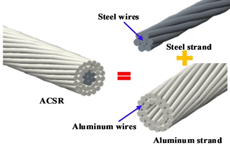
ACSR is a multi-stranded wire structure formed by concentric stranding of steel wires and aluminum wires, as shown in Fig. 1. During the operation of the transmission lines, ACSR can maintain a certain spatial shape after being pulled at the end along the axial direction [5]. Therefore, it has a certain bending rigidity, and the bending rigidity is closely related to the magnitude of the axial force [6]. Li et al. [7] researched the mechanical characteristics of the ACSR under axial load, and used the equivalent rigidity to solve the parameters such as the elastic modulus and Poisson’s ratio of the ACSR. However, there is not only squeezing between adjacent strands of ACSR, but also the transition between part of the strands from the adhesion state to the slip state [8]. As a result, the interaction between the internal strands of the ACSR is very complicated. The bending rigidity of the ACSR will not only depend on the axial force, but also on the contact state between the strands [9]. Wu et al. [10] and Dastous et al. [11] used the finite element method to analyze and calculate the internal contact problem of the stranded wire, which explained the change law of the static bending rigidity of the ACSR [12]. McConnell et al. [13] simplified the ACSR into an axial tension beam, established a calculation formula through theoretical derivation, and calculated the static bending rigidity of the ACSR based on the experimentally measured parameters such as axial force and vertical displacement.

The contact state between strands is complex under the action of dynamic load, which will directly affect the deformation state of ACSR. Therefore, the dynamic bending rigidity of ACSR becomes a problem that cannot be ignored. F. Lévesque et al. [14]-[15] presented experiments for the deformed shape of two types of ACSR undergoing vibrations, and gave the dynamic bending rigidity at different positions of the ACSR. S. Langlois et al. [16] modeled the deformed shape of the ACSR during aeolian vibrations using available bending rigidity models with a nonlinear time history finite element analysis. These studies on the dynamic load of ACSR point out the difference between the dynamic bending rigidity and the static bending rigidity of ACSR, which provides some reference for the research of this paper.

Fig. 1Structure diagram of ACSR

At present, most researches on the bending rigidity of ACSR focus on the static bending rigidity. Due to the complexity of the internal steel wires and aluminum wires of the ACSR under dynamic load, there is still a lack of relevant research on the calculation of the dynamic bending rigidity. Therefore, this paper designs a set of dynamic bending rigidity experiment device for ACSR, and taking one typical ACSR with different spans and different axial forces as object to study the variation rules of dynamic bending rigidity of ACSR. Finally, a comparative analysis of the dynamic bending rigidity and static bending rigidity of ACSR is given.

2. Theory of dynamic bending rigidity of ACSR

For a transmission line with rigidity and no damping, assume its rigidity as $E J$ , horizontal tension as $T_{0}$ , and the mass of per unit length is $m$ . The bending moment on the micro-element $d x$ , as shown in Fig. 2.

Fig. 2Vibration micro-element of ACSR

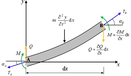
Based on the balance condition on the micro-element $d x$ , the balance equations ignored the high-order quantity can be derived as following:

1

\{\begin{array}{l} \sum F_{x} = 0, \begin{array}{l} T_{A} s i n α_{A} - T_{B} s i n α_{B} + m \frac{\partial^{2} y}{\partial t^{2}} d x + \frac{\partial Q}{\partial x} d x = 0, \end{array} \\ \sum \begin{array}{l} F_{y} = 0, \end{array} T_{A} c o s α_{A} = T_{B} c o s α_{B} = T_{0}, \\ \sum \begin{array}{l} M_{A} = 0, \end{array} \frac{\partial M}{\partial x} d x - Q d x = 0, \end{array}

where $T_{A}$ and $T_{B}$ are the tension of the ACSR at points A and B, respectively. $α_{A}$ and $α_{B}$ are the angles between the ACSR at points A and B and the horizontal direction ( $x$ -axis), respectively. $Q$ is the vertical force ( $y$ -axis) of the ACSR at point A.

The balance equations can be obtained from simplifying Eq. (1) as:

2

T_{0} \frac{\partial^{2} y}{\partial x^{2}} - m \frac{\partial^{2} y}{\partial t^{2}} - \frac{\partial Q}{\partial x} = 0,

3

\frac{\partial M}{\partial x} - Q = 0 .

Due to the effects of shear rigidity and rotational inertia are negligible when compared with the effects of bending rigidity [17], it can be known from the bending theory of Bernoulli-Euler beam theory that:

4

M = E J \frac{\partial^{2} y}{\partial x^{2}} .

Substituting Eq. (4) into Eq. (2-3), the following can be get:

5

Q = \frac{\partial M}{\partial x} = E J \frac{\partial^{3} y}{\partial x^{3}},

6

T_{0} \frac{\partial^{2} y}{\partial x^{2}} - m \frac{\partial^{2} y}{\partial t^{2}} - E J \frac{\partial^{4} y}{\partial x^{4}} = 0 .

Solve this partial differential equation with the method of separating variables, set $y (x, t) = U (x) ∙ V (t)$ , substituting Eq. (6) can get:

7

E J \frac{1}{m U} \frac{d^{4} y}{d x^{4}} - \frac{T_{0}}{m U} \frac{d^{2} y}{d x^{2}} = - \frac{1}{V} \frac{d^{2} V}{d t^{2}} .

Eq. (7) is the function of $x$ on the left and the function of $t$ on the right. The left and right sides must be equal to the same constant. Suppose this constant is $ω^{2}$ , and two ordinary differential equations can be obtained:

8

E J \frac{1}{m U} \frac{d^{4} U}{d x^{4}} - \frac{T_{0}}{m U} \frac{d^{2} U}{d x^{2}} = m U ω^{2},

9

\frac{d^{2} V}{d t^{2}} = - V ω^{2} .

The solution of Eq. (8) is:

10

V (t) = A s i n ω t + B c o s ω t .

Assuming that the two ends of the ACSR are hinged, the boundary conditions are:

11

\{\begin{array}{l} U (0) = 0, \begin{array}{l} \frac{d^{2} U (0)}{d x^{2}} = 0, \end{array} \\ U (l) = 0, \begin{array}{l} \frac{d^{2} U (l)}{d x^{2}} = 0, \end{array} \end{array}

where $l$ is the span of the ACSR.

According to Eq. (11), the form of $U (x)$ can be set as:

12

U (x) = U s i n \frac{n π x}{l} \begin{array}{l} , & (n = 1,2, 3 \dots) \end{array} .

Substituting Eq. (12) into Eq. (8), the following can be get:

13

E J {(\frac{n π}{l})}^{4} s i n \frac{n π x}{l} + T_{0} {(\frac{n π}{l})}^{2} s i n \frac{n π x}{l} = m ω^{2} s i n \frac{n π x}{l} .

Therefore, the natural frequency of the hinged beam at both ends with the axial force is:

14

ω_{n} = {(\frac{n π}{l})}^{2} \sqrt{\frac{E J}{m}} \sqrt{1 + \frac{T_{0} l^{2}}{n^{2} π^{2} E J}} .

When $T_{0} =$ 0, the first natural frequency of the hinged beam at both ends with the axial force from Eq. (14) is:

15

ω_{1}^{0} = {(\frac{π}{l})}^{2} \sqrt{\frac{E J}{m}} .

For the hinged beam at both ends, the axial force influence coefficient of the first natural frequency is:

16

α_{1} = \frac{ω_{1}}{ω_{1}^{0}} = \sqrt{1 + \frac{T_{0}}{T_{1}^{c r}}},

where $T_{1}^{c r}$ is the first-order Euler critical force.

When $- 0.5 T_{1}^{c r} \leq T_{0} \leq 0.5 T_{1}^{c r}$ , for a constant-section beam with stable support, the maximum relative error of the axial force influence coefficient obtained by Eq. (16) does not exceed 2 % [18].

Timoshenko gave the first-order Euler critical force of a fixed beam at both ends as [19]:

17

T_{1}^{c r} = \frac{4 π^{2} E J}{l^{2}} .

Substituting Eq. (15) and Eq. (17) into Eq. (16), the bending rigidity of the beams fixed at both ends can be expressed as:

18

E J = \frac{ω_{1}^{2} l^{4} m}{π^{4}} - \frac{T_{0} l^{2}}{4 π^{2}} .

It can be seen from Eq. (18) that under the conditions of fixed axial load and pitch, the dynamic bending rigidity of ACSR can be measured by the natural frequency of the structure. Therefore, the solution of the dynamic bending rigidity of ACSR is transformed into the measurement of its natural frequency.

3. Experiment on dynamic bending rigidity of ACSR

In this study, the white noise excitation and hammer excitation methods are used to study the dynamic response of ACSR. The dynamic bending rigidity of the ACSR under different spans and different axial forces is obtained, and the changing rules of the dynamic bending rigidity is given.

3.1. Specimens details

In this experiment, the typical JL/G1A-300/25-48/7 ACSR [20] was selected as the experimental specimens, and the parameters of JL/G1A-300/25-48/7 ACSR are shown in Fig. 3 and Table 1. The twisting pitch of the outer stranded wire of JL/G1A-300/25-48/7 is 330 mm. In order to avoid the ACSR is too short, the span of the experimental ACSR is not less than 2 times the pitch. Therefore, the experimental span selected in the experiment process of this article are 870 mm, 1020 mm, 1170 mm, 1320 mm, 1470 mm and 1620 mm respectively.

Fig. 3Diagram of experimental ACSR

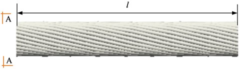
a) JL/G1A-300/25-48/7 ACSR

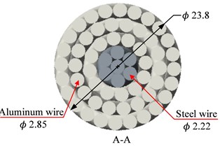
b) Section A-A

Table 1Parameters of ACSR JL/G1A-300/25-48/7

Cross-sectional area of Aluminum/Steel (mm²)	Number/Diameter (mm)		Calculated cross-sectional area A (mm²)			Outer diameter $d$ (mm)	Breaking force $T_{j}$ (N)	Allowable stress $δ_{0}$ (MPa)	Linear mass $m$ (kg/km)
	Aluminum	Steel	Aluminum	Steel	Total
300/25	48/2.85	7/2.22	306	27.1	333	23.8	83760	95.1	1057.9

3.2. Experimental setup, instrumentation, and loading protocol

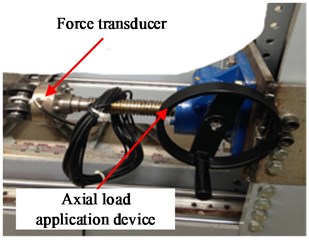
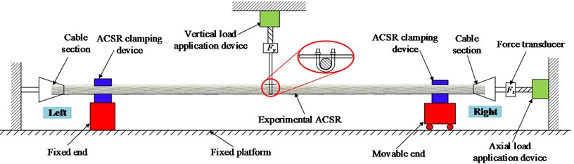
The experimental device is composed of axial load application device, ACSR clamping force application device, cable section and excitation device, as shown in Fig. 4(a) and Fig. 4(b). The left end of the experimental ACSR is a fixed end, and the right end is movable, which can move along the slide rail equipped with the fixed platform. In order to limit the movement of the ACSR, a ACSR clamping device with upper and lower clamping blocks was designed as shown in Fig. 5. The upper and lower surfaces of the clamps are milled with circular grooves that match the shape of the ACSR, and the clamps are connected by bolts.

In the experiment, it is necessary to simulate the tensile force of the ACSR in service, which made the strands of the intercepted wire have close contact without separation. Therefore, the cable section in Fig. 5 are used to fix both ends of the wire. The axial force application device of ACSR is shown in Fig. 6, which is composed of a force transducer and a stretching device rotated by a hand wheel. The axial force applied to the end of the ACSR is controlled by rotating the handle. With reference to the actual axial load of the ACSR in service, this study takes the maximum axial tension as 15 kN and the minimum axial tension as 3 kN. The value of the axial tension in the experiment starts from 3 kN, and a set of data is recorded every 2 kN.

Fig. 4Experimental device

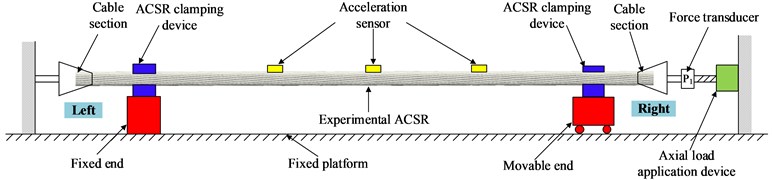
a) Schematic diagram of experimental device

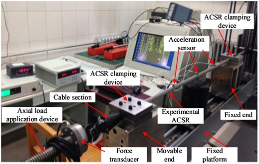
b) Layout of the experimental device

Fig. 5Cable section and clamping device

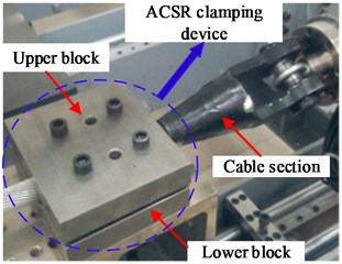
Fig. 6Axial load application device

3.3. Excitation system for dynamic bending rigidity experiment

According to the theory of dynamic bending rigidity of ACSR, it is necessary to obtain the natural frequency to get the dynamic bending rigidity of ACSR. In the experiment, both ends of the ACSR are set as fixed constraints, and the axial load is applied to the ACSR. Two methods of white noise excitation and force hammer excitation are used to obtain the natural frequency of the ACSR, and then the dynamic bending rigidity of the ACSR is obtained.

3.3.1. White noise excitation

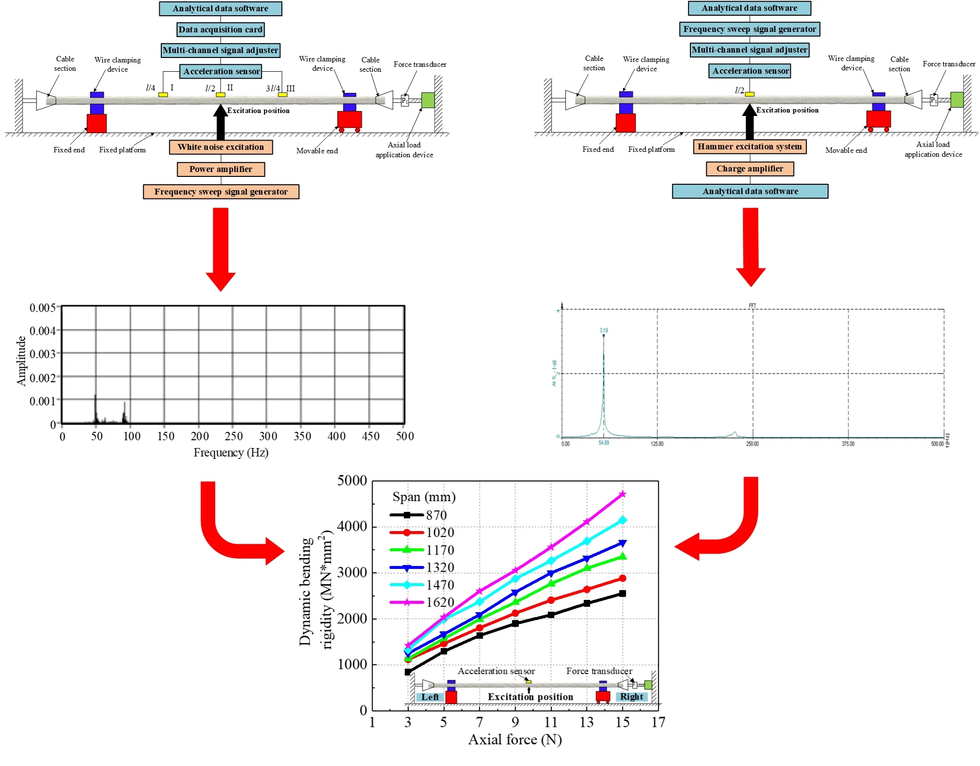
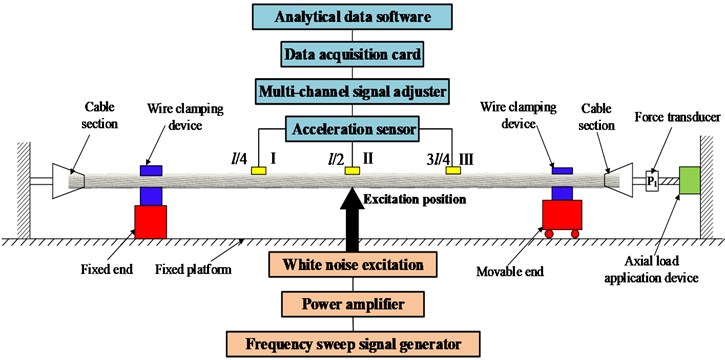
Fig. 7 shows a white noise excitation system, in which the exciter is connected to the experimental ACSR through the ejector rod to provide an excitation force. The frequency sweep signal generator can generate random signals, which can be used as the signal source of the vibration exciter. The power amplifier can amplify the random signal generated by the sweep signal generator and use it as the input signal of the vibration exciter to complete the vibration excitation of the test. There are three acceleration sensors are set at $l$ /4, $l$ /2 and 3 $l$ /4 on the ACSR to collect vibration response signals. A multi-channel signal adjuster is used with the acceleration sensor to filter and amplify the measured acceleration signal. The data acquisition card can digitize and discretize the obtained analog signal, which can then be analyzed and processed by subsequent software.

In this experiment, the excitation position is the middle position of the ACSR and the different pitches and axial force of ACSR are selected. The vibration signal is collected through the data acquisition card and connected to the computer data processing software. The collected vibration of time domain signal is transformed into frequency domain signal by Fast Fourier Transform (FFT), which is used for self-cross spectrum analysis to obtain the natural frequency of the ACSR.

Fig. 7Schematic diagram of white noise excitation system

3.3.2. Hammer excitation

Fig. 8 shows the hammer excitation system. The charge amplifier cooperates with the piezoelectric sensor on the force hammer to measure mechanical vibration or shock pressure. The filter of the charge amplifier can filter out the folding distortion and unwanted high-frequency components in the vibration response of the ACSR after being hammered, and accurately determine the strength of the hammer signal. The data acquisition and processing also use the multi-channel signal conditioning instrument and the change of frequency domain signal by FFT in the white noise excitation.

Fig. 8Schematic diagram of hammer excitation system

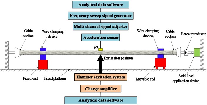
In the hammer excitation experiment, the acceleration sensor is located at $l$ /2 of the ACSR and the different pitches and axial force are applied. The excitation position is the middle position of the ACSR. The time-domain and frequency-domain diagrams of the hammer can judge whether the method and strength of the percussion are reasonable. The collected vibration time-domain signal is transformed into frequency-domain signal by FFT, and the natural frequency of ACSR is obtained by the traditional peak method.

4. Experimental results

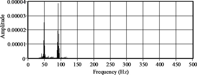
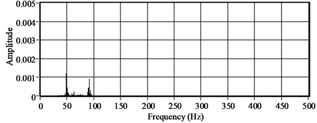
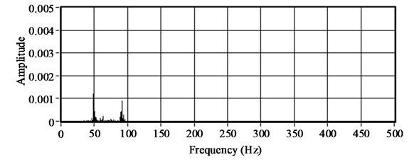
The vibration response signal can be analyzed by self-power spectrum and cross-power spectrum analysis with mean value treatment to obtain the natural frequency of the ACSR. Take the vibration signal of the ACSR with a span of 1320 mm and an axial tension of 11 kN as an example, the self-power spectrum diagram of channels one to three get from acceleration sensor I to III by FFT are shown in Fig. 9. Fig. 10 shows the cross-power spectrum diagram of the second channel and other channels according to the method of self-cross spectrum power. It can be found from the self-power spectrum of each channel and the cross-power spectrum diagram that the first natural frequency of the ACSR with a span of 1320 mm and an axial tension of 11 kN is about 49.95 Hz.

Fig. 9Self-power spectrum of channels

a) Channel one

b) Channel two

c) Channel three

Fig. 10Cross-power spectrum of reference channel and other channels

a) Channel two and channel one

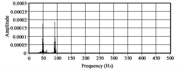
b) Channel two and channel three

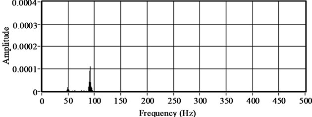
The force hammer excitation recognizes the dynamic parameters by collecting the time domain signal and the frequency response function obtained by the output response. Fig. 11 shows the natural frequency analysis diagram of the ACSR obtained by the traditional Peak-Picking method with a span of 1320 mm and an axial tension of 11 kN.

Fig. 11Signals and frequency spectrum of exciting cantilever beam (l= 1320 mm, T0= 11 kN)

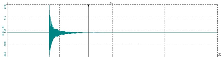
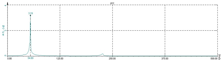
In Fig. 11, after the vibration signal is transformed by FFT, the frequency at the peak is the natural frequency of the ACSR, and the analyzed frequency is about 51.76 Hz. It can be found that the natural frequency of the ACSR obtained by white noise and hammer excitation are 49.95 Hz and 51.76 Hz, respectively, and the relative error is less than 4 %. In this study, the frequency obtained by the force hammer excitation is used to substitute the Eq. (18) to calculate the dynamic bending rigidity of ACSR. Fig. 12 shows the change law of the dynamic bending rigidity of the ACSR with the axial force under the six experimental spans. It can be found that the dynamic bending rigidity of the ACSR is greatly affected by the axial force. The greater the axial force, the greater the dynamic bending rigidity. Table 2 shows the dynamic bending rigidity and the first natural frequency of the ACSR with different spans and different axial force.

Fig. 12Dynamic bending rigidity of ACSR

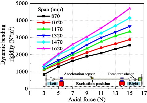
Table 2Dynamic bending rigidity and the first natural frequency of ACSR

$l$ (mm)	870		1020		1170		1320		1470		1620
$T_{0}$ (kN)	$ω_{1}$ (Hz)	$E J$ (N∙m²)	$ω_{1}$ (Hz)	$E J$ (N∙m²)	$ω_{1}$ (Hz)	$E J$ (N∙m²)	$ω_{1}$ (Hz)	$E J$ (N∙m²)	$ω_{1}$ (Hz)	$E J$ (N∙m²)	$ω_{1}$ (Hz)	$E J$ (N∙m²)
3	60.55	844.4	50.78	1119.4	41.02	1138.0	32.25	1250.2	27.34	1332.1	23.44	1423.5
5	75.20	1295.4	58.59	1464.3	47.85	1571.6	37.11	1670.0	33.20	1993.4	28.32	2037.5
7	84.96	1641.8	65.43	1806.4	52.73	1996.5	42.97	2094.3	37.11	2375.3	32.23	2604.9
9	91.80	1901.3	71.29	2126.6	57.62	2362.1	47.85	2583.2	41.02	2878.2	35.16	3056.4
11	96.68	2089.9	76.17	2409.2	62.50	2765.6	51.76	3002.8	43.95	3268.8	38.09	3559.3
13	102.54	2339.1	80.08	2641.1	66.41	3102.6	54.69	3321.3	46.88	3693.2	41.02	4112.0
15	107.42	2553.2	83.98	2886.5	69.34	3354.3	57.62	3662.0	49.80	4149.8	43.95	4715.3
Note: $l$ is the span of the experimental ACSR, $T_{0}$ is the axial force applied to the experimental ACSR, $ω_{1}$ is the first natural frequency of the experimental ACSR and $E J$ is the dynamic bending rigidity of the experimental ACSR.

5. Comparison and discussion

5.1. The influence of axial force and span on dynamic bending rigidity

It can be concluded that the dynamic bending rigidity of the ACSR is affected by the axial force and span from the experimental results in the previous section. Table 3 shows the rigidity ratio of the same span relative to axial force is 3 kN and the rigidity ratio of the same axial force relative to span is 870 mm. It can be found that with the same span, the dynamic bending rigidity ratio of the ACSR increases from 1.0 to 3.0 as the axial increases, and the value in each level of axial force is almost the same. The possible reason is the increase in axial force makes the strands inside the ACSR more closely contact each other, which leads to an increase in the overall rigidity. On the other aspect, the dynamic bending rigidity of the ACSR increases significantly with the increase of the span. With the same axial force, the dynamic bending rigidity ratio of the ACSR increases from 1.0 to 1.6 as the span increases, and the value in each level of span is also almost the same. This may be caused by the weight of the ACSR increases as the span becomes larger, and therefore the vibration amplitude becomes smaller under the output power of the exciter remains unchanged. Hence, the resulting dynamic bending rigidity is relatively increased.

Table 3Rigidity ratio of the same span relative to T0= 3 kN and the same axial force relative to l= 870 mm

$T_{0}$ (kN)	Rigidity ratio of the same span / Rigidity ratio of the same axial force
3	1.0/1.0	1.0/1.3	1.0/1.3	1.0/1.5	1.0/1.6	1.0/1.7
5	1.5/1.0	1.3/1.1	1.4/1.2	1.3/1.3	1.5/1.5	1.4/1.6
7	1.9/1.0	1.6/1.1	1.8/1.2	1.7/1.3	1.8/1.4	1.8/1.6
9	2.3/1.0	1.9/1.1	2.1/1.2	2.1/1.4	2.2/1.5	2.1/1.6
11	2.5/1.0	2.2/1.2	2.4 /1.3	2.4/1.4	2.5/1.6	2.5/1.7
13	2.8/1.0	2.4/1.1	2.7/1.3	2.7/1.4	2.8/1.6	2.9/1.8
15	3.0/1.0	2.6/1.1	2.9/1.3	2.9/1.4	3.1/1.6	3.3/1.8

5.2. Comparison with the static bending rigidity

The static bending rigidity of the ACSR is the ability to resist bending deformation under static load. The schematic diagram of the test device for measuring the static bending rigidity of the ACSR is shown in Fig. 13 [2]. Similar to the dynamic bending rigidity experimental device, a transverse load is applied after the ACSR is clamped, and a vertical load is applied to the middle of the ACSR. The calculation equation of the static bending rigidity of ACSR is [2]:

19

E I = \frac{F_{x} l^{2}}{4 λ^{2}},

where $E I$ is the static bending rigidity of the ACSR, $F_{x}$ is the axial force of ACSR, $l$ is the span of ACSR, and the equation that $λ$ needs to satisfy is:

20

\frac{4 F_{x} Δ}{F_{y} l} = 1 + \frac{2 (1 - c o s h λ)}{λ s i n h λ},

where $F_{y}$ is the vertical force applied on the middle of the ACSR, and $Δ$ is the displacement in the mid-span of the ACSR.

Fig. 13Schematic diagram of the experimental device for the static bending rigidity of the ACSR

It can be found that the static bending rigidity of the ACSR is related to the vertical force from Eqs. (19-20). The static bending rigidity of the ACSR in the literature is also obtained under different vertical loads [2]. Table 4 and Table 5 show the static bending rigidity of the ACSR and the ratio of dynamic bending rigidity to the static bending rigidity when the span is 870 mm and 1020 mm with five axial and vertical force. The dynamic bending rigidity is calculated by getting or interpolating the value at the corresponding position according to the results of the previous section.

It can be concluded from Table 4 and Table 5 that under the same vertical load, the change law of the static bending rigidity and dynamic bending rigidity of the ACSR is basically the same, that is, the greater the axial force, the greater the bending rigidity. When the axial force is constant, the static bending rigidity of the ACSR increases with the decrease of the vertical load. This is because the smaller vertical load makes the bending deformation of the ACSR smaller, and the viscous effect between the strands is enhanced, which caused the static bending rigidity is larger. However, even when the static bending rigidity is maximum, the dynamic bending rigidity is more than 7 times the static bending rigidity, which also means that the dynamic bending rigidity of the ACSR is closer to the value by assuming a “solid body” (welded strand to strand) behavior in literature [13]. In addition, when the axial force was increased from 3 kN to 15 kN, the ratio of dynamic bending rigidity to static bending rigidity of the ACSR at two spans decreased by 50 % and 70 %, respectively. It indicates that the increase of the axial force has a greater effect on the static bending rigidity of the ACSR than the dynamic bending rigidity, and the increase of the span will aggravate this effect.

Table 4The static bending rigidity and the ratio at the span of 870 mm

$F_{x}$ (kN)	3		6		9		12		15
$F_{y}$ (kN)	$E I$ (N∙m²)	Ratio	$E I$ (N∙m²)	Ratio	$E I$ (N∙m²)	$F_{y}$ (kN)	$E I$ (N∙m²)	Ratio	$E I$ (N∙m²)	Ratio
0.1	40	21	86	17	176	11	194	11	261	10
0.2	22	38	48	31	107	18	135	16	198	13
0.3	18	47	33	45	70	27	89	25	170	15
0.4	13	65	27	54	53	36	73	30	133	19
0.5	11	77	20	73	38	50	56	40	110	23

Table 5The static bending rigidity and the ratio at the span of 1020 mm

$F_{x}$ (kN)	3		6		9		12		15
$F_{y}$ (kN)	$E I$ (N∙m²)	Ratio	$E I$ (N∙m²)	Ratio	$E I$ (N∙m²)	Ratio	$E I$ (N∙m²)	Ratio	$E I$ (N∙m²)	Ratio
0.1	37	23	84	17	171	11	201	11	358	7
0.2	20	42	42	35	87	22	127	17	226	11
0.3	16	53	27	54	51	37	93	24	156	16
0.4	13	65	18	62	31	61	63	35	130	20
0.5	10	84	14	80	24	79	46	48	107	24

6. Conclusions

The dynamic bending rigidity of ACSR is a key parameter for dynamic response analysis of overhead transmission lines. This paper derives the calculation formula for the dynamic bending rigidity of the ACSR, and designs a set of experimental equipment for the dynamic bending rigidity of the ACSR. The principle of the experimental device is simple and clear, and the vibration frequency of the ACSR can be obtained more accurately. Through the analysis of the experimental results of the dynamic bending rigidity of ACSR with different spans and different axial forces, the following conclusions can be drawn:

1) Similar to the static bending rigidity, the dynamic bending rigidity of the ACSR will increase with the increase of the axial force and the span, and the growth rate is almost the same.

2) The dynamic bending rigidity is more than 7 times the static bending rigidity, that is, the dynamic bending rigidity of the ACSR is much greater than the static bending rigidity. Therefore, when conducting dynamic analysis of the ACSR, the change of its rigidity should be considered.

3) The increase of the axial force has a greater effect on the static bending rigidity of the ACSR than the dynamic bending rigidity, and the increase of the span will aggravate this effect.

References

X. L. Gong, “Experimental research on bending rigidity of overhead line,” (in Chinese), M.A. Thesis, North China Electric Power University, 2013.

Search CrossRef
G. F. Yang, “The study on the equivalent bending rigidity of ACSR,” (in Chinese), M.A. Thesis, North China Electric Power University, 2014.

Search CrossRef
Z. Wang, L. Qi, W. Yang, and M. Wang, “Research on the applicability of lumped mass method for cable’s dynamic tension in the ice shedding experiment,” (in Chinese), Zhongguo Dianji Gongcheng Xuebao/Proceedings of the Chinese Society of Electrical Engineering, Vol. 34, No. 12, p. 2014, 1982, https://doi.org/10.13334/j.0258-8013.pcsee.2014.12.019

Publisher
L. Qin, L. Ya-Nan, and X. G. Wei, “Nonlinear numerical simulation for galloping of single iced conductor,” (in Chinese), Science Technology and Engineering, Vol. 14, No. 4, pp. 230–235, 2014.

Search CrossRef
N. C. Perkins and C. D. Mote, “Three-dimensional vibration of travelling elastic cables,” Journal of Sound and Vibration, Vol. 114, No. 2, pp. 325–340, 1987.

Publisher
F. Baron and M. S. Venkatesan, “Nonlinear analysis of cable and truss structures,” Journal of the Structural Division, Vol. 97, No. 2, pp. 679–710, Feb. 1971, https://doi.org/10.1061/jsdeag.0002824

Publisher
L. Yongping, Z. Yi, S. Pan, H. Zhiyi, and N. Yang, “Study on section stiffness, Poisson ratio and mechanism characteristics of large cross-sectional aluminum-steel stranded conductor,” Energy Procedia, Vol. 17, pp. 843–850, 2012, https://doi.org/10.1016/j.egypro.2012.02.178

Publisher
K.-J. Hong, A. der Kiureghian, and J. L. Sackman, “Bending behavior of helically wrapped cables,” Journal of Engineering Mechanics, Vol. 131, No. 5, pp. 500–511, May 2005, https://doi.org/10.1061/(asce)0733-9399(2005)131:5(500)

Publisher
K. Inagaki, “Mechanical models for electrical cables,” Royal Institute of Technology KTH Mechanics, Sweden, 2005.

Search CrossRef
Q. Wu, K. Takahashi, and S. Nakamura, “Non-linear vibrations of cables considering loosening,” Journal of Sound and Vibration, Vol. 261, No. 3, pp. 385–402, Mar. 2003, https://doi.org/10.1016/s0022-460x(02)01090-8

Publisher
J. B. Dastous, “Nonlinear finite-element analysis of stranded conductors with variable bending stiffness using the tangent stiffness method,” IEEE Transactions on Power Delivery, Vol. 20, No. 1, pp. 328–338, Jan. 2005, https://doi.org/10.1109/tpwrd.2004.835420

Publisher
K. O. Papailiou, “On the bending stiffness of transmission line conductors,” IEEE Transactions on Power Delivery, Vol. 12, No. 4, pp. 1576–1588, 1997, https://doi.org/10.1109/61.634178

Publisher
K. G. Mcconnell and W. P. Zemke, “The measurement of flexural stiffness of multistranded electrical conductors while under tension,” Experimental Mechanics, Vol. 20, No. 6, pp. 198–204, Jun. 1980, https://doi.org/10.1007/bf02327599

Publisher
F. Levesque, S. Goudreau, S. Langlois, and F. Legeron, “Experimental study of dynamic bending stiffness of ACSR overhead conductors,” IEEE Transactions on Power Delivery, Vol. 30, No. 5, pp. 2252–2259, Oct. 2015, https://doi.org/10.1109/tpwrd.2015.2424291

Publisher
F. Levesque, S. Goudreau, S. Langlois, and F. Legeron, “Experimental study of dynamic bending stiffness of ACSR drake overhead conductor,” in International Symposium on Cable Dynamics, 2011.

Search CrossRef
S. Langlois, F. Legeron, and F. Levesque, “Time history modeling of vibrations on overhead conductors with variable bending stiffness,” IEEE Transactions on Power Delivery, Vol. 29, No. 2, pp. 607–614, 2014, https://doi.org/10.1109/tpwrd.2013.2279604

Publisher
R. A. Sousa, R. M. Souza, F. P. Figueiredo, and I. F. M. Menezes, “The influence of bending and shear stiffness and rotational inertia in vibrations of cables: An analytical approach,” Engineering Structures, Vol. 33, No. 3, pp. 689–695, Mar. 2011, https://doi.org/10.1016/j.engstruct.2010.11.026

Publisher
G. Y. Zhang, H. S. Zhang, and N. L. Lu, “The axial load influence coefficient of natural frequencies for lateral vibration of a Bernoulli-Euler beam,” (in Chinese), Engineering Mechanics, Vol. 28, No. 10, pp. 65–71, 2011.

Search CrossRef
W. Weaver, S. P. Timoshenko, and H. D. Young, Vibration Problems in Engineering. Wiley, 1974.

Search CrossRef
“GB/T 1179-2017 Round wire concentric lay overhead electrical stranded conductors,” China Standard Press, Beijing, General Administration of Quality Supervision, Inspection and Quarantine of the People’s Republic of China, China National Standardization Management Committee, 2017.

Search CrossRef

About this article

Received

05 April 2022

Accepted

22 June 2022

Published

24 July 2022

SUBJECTS

Mechanical vibrations and applications

DOI

https://doi.org/10.21595/jve.2022.22573

Keywords

aluminium cable steel reinforced (ACSR)

Bernoulli-Euler beam

dynamic bending rigidity

experimental study

Acknowledgements

The authors are grateful for the financial support provided by the Science and Technology Program of Baoding [No. 1911ZG019].

This is an open access article distributed under the Creative Commons Attribution License, which permits unrestricted use, distribution, and reproduction in any medium, provided the original work is properly cited.

Previous article in issue Previous Next article in issue Next

Research article

2023 08 03

Experimental analysis on the structural seismic behavior of steel frame-precast steel reinforced concrete (SRC) infill wall with lateral force resisting

Xiaohui Wang, Hui Zhang, Xiaolong Hu

Research article

2020 05 15

Two-span bridge under moving load – numerical and experimental approach

Veronika Valašková, Daniela Kuchárová, Jozef Melcer

Research article

2018 09 30

Analytical solution for modal analysis of Euler-Bernoulli and Timoshenko beam with an arbitrary varying cross-section

Fatemeh Sohani, H. R. Eipakchi

Research article

2016 11 15

Experimental research and numerical simulation of influence of pre-stress values on the natural vibration frequency of concrete simply supported beams

Jie Li, Feng Zhang

K. Hao, Z. Mo, and S. Lu, “Experimental study on dynamic bending rigidity of aluminium cable steel reinforced,” Journal of Vibroengineering, Vol. 24, No. 7, pp. 1235–1248, Jul. 2022, https://doi.org/10.21595/jve.2022.22573

Copy Extrica

Copied to clipboard!

TY  - JOUR
DO  - 10.21595/jve.2022.22573
UR  - https://doi.org/10.21595/jve.2022.22573
TI  - Experimental study on dynamic bending rigidity of aluminium cable steel reinforced
T2  - Journal of Vibroengineering
AU  - Hao, Keming
AU  - Mo, Ze
AU  - Lu, Siyao
PY  - 2022
DA  - 2022/07/24
PB  - JVE International Ltd.
SP  - 1235-1248
VL  - 24
IS  - 7
SN  - 1392-8716
SN  - 2538-8460
ER  - 

Copy Ris

Copied to clipboard!

@article{Hao_2022,
	doi = {10.21595/jve.2022.22573},
	url = {https://doi.org/10.21595/jve.2022.22573},
	year = 2022,
	month = {jul},
	publisher = {{JVE} International Ltd.},
	volume = {24},
	number = {7},
	pages = {1235--1248},
	author = {Keming Hao and Ze Mo and Siyao Lu},
	title = {Experimental study on dynamic bending rigidity of aluminium cable steel reinforced},
	journal = {Journal of Vibroengineering}
}

Copy Bibtex

Copied to clipboard!

[1]K. Hao, Z. Mo, and S. Lu, “Experimental study on dynamic bending rigidity of aluminium cable steel reinforced,” Journal of Vibroengineering, vol. 24, no. 7, pp. 1235–1248, Jul. 2022, doi: 10.21595/jve.2022.22573.

Copy IEEE

Copied to clipboard!

Hao, Keming, Ze Mo, and Siyao Lu. “Experimental Study on Dynamic Bending Rigidity of Aluminium Cable Steel Reinforced.” Journal of Vibroengineering 24, no. 7 (July 24, 2022): 1235–48. https://doi.org/10.21595/jve.2022.22573.

Copy Chicago

Copied to clipboard!

Experimental study on dynamic bending rigidity of aluminium cable steel reinforced

Abstract

Highlights

1. Introduction

2. Theory of dynamic bending rigidity of ACSR

3. Experiment on dynamic bending rigidity of ACSR

3.1. Specimens details

3.2. Experimental setup, instrumentation, and loading protocol

3.3. Excitation system for dynamic bending rigidity experiment

3.3.1. White noise excitation

3.3.2. Hammer excitation

4. Experimental results

5. Comparison and discussion

5.1. The influence of axial force and span on dynamic bending rigidity

5.2. Comparison with the static bending rigidity

6. Conclusions

References

About this article

Related Articles