Two-span bridge under moving load – numerical and experimental approach

1. Introduction

The moving load on bridges is one of the most important components of the load. Simulation of moving load effect on bridges was induced by the collapse of the Chester Rail Bridge in England in the year 1847 and it can be traced in the literature since the year 1849, [1, 2]. The authors as V. Koloušek [3] and L. Frýba [4] laid the foundations to the deep tradition of modeling of moving load effects on transport structures. Their work obtained world acknowledgment. To the dynamic of railway and highway bridges are especially dedicated the monographs [5, 6]. While the problem of the dynamic of railway bridges was studied since the year 1847, the problems of dynamic of highway bridges start to be studied only in the 20th century. American Society of Civil Engineers in [7] published the 1st important report on this topic. The complete overview of the works in this area until the year 1975 was published by Tseng Huang in [8]. New findings to the solution of the problem can be found for example in [9-12]. A numerical approach to the solution of the vehicle-bridge interaction problems requires to pay attention to the following matters: creating the vehicle and the bridge computational models, creating the computing programs for the solution of equations of motion and displaying of obtained results. To solve this problem, it is advantageous to work with discrete computational models. Computational models can be created from the spirit of classical dynamics or in the spirit of the finite element method. When working with the finite element method, it is advisable to use the ADYNA or ANSYS program systems [13-15]. Classic computational models can be advantageously solved in the environment of the program system MATLAB [16]. This contribution is devoted to the numerical modeling of vehicle movement over the two-span highway bridge on the basis of two approaches (FEM and classical approach). It described the creation of a discrete computational model of the vehicle and a bridge. The time courses of vehicle and bridge oscillation are shown graphically. Important results are given in the numerical form.

2. Computational models of a bridge

The subject of numerical analysis is a highway bridge with two fields. It is a prestressed concrete bridge made of I-73 bridge prefabricated elements. Planar models of a bridge are often used in practical engineering tasks. For the purpose of this paper, the bridge is modeled as a Bernoulli-Euler continuous beam with two fields. Two models are created for the solution of this task. One model is based on classical dynamics and the other is based on the finite element method.

2.1. Model-based on classical dynamics

The bridge model based on classical dynamics is a discrete computational model with two degrees of freedom, Fig. 1. One application of such a computational model was already introduced in [17]. We need to solve two problems when we want to use such a computational model. We must adopt the assumption about the shape of the deflection curve, the function ${\mathrm{\Phi }}_v\left(x\right)$, and define the load distribution function ${\mathrm{\Phi }}_F\left(x\right)$. The functions ${\mathrm{\Phi }}_v\left(x\right)$ and ${\mathrm{\Phi }}_F\left(x\right)$ can be linear, sinusoidal or parabolic. Numerical studies show that the best results are obtained if the function ${\mathrm{\Phi }}_v\left(x\right)$ is sinusoidal and the function ${\mathrm{\Phi }}_F\left(x\right)$ is linear, as it is seen in Fig. 1.

Fig. 1Computational model of a bridge with two degrees of freedom

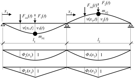
The equations of motion describing such computational model are as follows:

1

${\ddot{v}}_1\left(t\right)\bullet m_{b1}+2{\omega }_b\bullet {\dot{v}}_1\left(t\right)+k_{11}\bullet v_1\left(t\right)+k_{12}\bullet v_2\left(t\right)=F_1\left(t\right),$
${\ddot{v}}_2\left(t\right)\bullet m_{b2}+2{\omega }_b\bullet {\dot{v}}_2\left(t\right)+k_{21}\bullet v_1\left(t\right)+k_{22}\bullet v_2\left(t\right)=F_2\left(t\right),$

where ${\omega }_b$is the damping circular frequency in rad/s and $k_{ij}$ are the stiffness constants in N/m.

The load distribution function is defined as:

2

$0\le x_1\le \frac{l_1}{2},{\mathrm{\Phi }}_F\left(x_1\right)=\frac{2}{l_1}{x}_1,\frac{l_1}{2}\le x_1\le l_1,{\mathrm{\Phi }}_F\left(x_1\right)=\frac{2}{l_1}{(l_1-x}_1),$
$0\le x_2\le \frac{l_2}{2},{\mathrm{\Phi }}_F\left(x_2\right)=\frac{2}{l_2}{x}_2,\frac{l_2}{2}\le x_2\le l_2,{\mathrm{\Phi }}_F\left(x_2\right)=\frac{2}{l_2}{(l_2-x}_2).$

Approximation of the deflection curve can be described as:

3

$v\left(x_1,t\right)={\mathrm{\Phi }}_v\left(x_1\right)\bullet v_1\left(t\right)+u\left(x\right),v_{x1}\left(t\right)={\mathrm{\Phi }}_v\left(t\right)\bullet v_1\left(t\right)+u\left(t\right),$
$v\left(x_2,t\right)={\mathrm{\Phi }}_v\left(x_2\right)\bullet v_2\left(t\right)+u\left(x\right),v_{x2}\left(t\right)={\mathrm{\Phi }}_v\left(t\right)\bullet v_2\left(t\right)+u\left(t\right),$

where the shape function ${\mathrm{\Phi }}_v\left(x\right)$ is defined as:

4

${\mathrm{\Phi }}_v\left(x_1\right)=\mathrm{s}\mathrm{i}\mathrm{n}\left(\frac{\pi \bullet x_1}{l_1}\right),{\mathrm{\Phi }}_v\left(x_2\right)=\mathrm{s}\mathrm{i}\mathrm{n}\left(\frac{\pi \bullet x_2}{2}\right).$

Function $u\left(x\right)$ represents the road unevenness. In relation to the particular vehicle speed the functions $u$, ${\mathrm{\Phi }}_v$, ${\mathrm{\Phi }}_F$ can be expressed as functions of time $t$. For example:

5

${\mathrm{\Phi }}_v\left(x\right)=\mathrm{s}\mathrm{i}\mathrm{n}\left(\frac{\pi \bullet x}{l}\right),{\mathrm{\Phi }}_v\left(t\right)=\mathrm{s}\mathrm{i}\mathrm{n}\left(\frac{\pi \bullet e\bullet t}{l}\right)=\sin \left(\omega \bullet t\right),\omega =\pi \bullet \frac{e}{l},$

6

${\mathrm{\Phi }}_F\left(x\right)=\frac{2}{l}x,{\mathrm{\Phi }}_F\left(t\right)=\frac{2}{l}e\bullet t,$
${\mathrm{\Phi }}_F\left(x\right)=\frac{2}{l}\left(l-x\right),{\mathrm{\Phi }}_F\left(t\right)=\frac{2}{l}\left(l-e\bullet t\right),$

where e is the vehicle speed in m/s.

The force $F\left(t\right)$ acting on the mass point $m_b$ at time $t$ can be expressed as:

7

$F\left(t\right)=F_{int}\left(t\right)\bullet {\mathrm{\Phi }}_F\left(t\right).$

Derivatives of functions with respect to time are denoted by a dot above the symbol.

3. Computational model of a vehicle

For the purpose of this paper the half planar computational model of the lorry Tatra 815 was adopted, Fig. 2. It is a discrete computational model with eight degrees of freedom [19]. The five degrees of freedom are mass and the three degrees of freedom are mass-less.

Fig. 2Two-dimensional computational model of Tatra 815 lorry

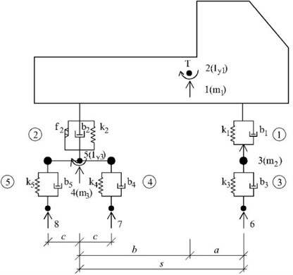
Equations of motion for five unknown functions $r_1\left(t\right)$-$r_5\left(t\right)$ describing the vehicle vibration and corresponding to displacements of mass degrees of freedom are derived as ordinary differential Eq. (9):

The contact forces $F_{int,i}$ ($i=$ 6, 7, 8) belong to individual contact points are expressed as:

In the above equations $k$, $b$, $m$ are stiffness, damping and mass characteristics of the vehicle model and $G$ is the gravity force. The dot about the symbol marks derivative with respect to time $t$.

The computational model of vehicle in ADINA is a discrete computational model. The model is consists of beam elements with high bending stiffness and mass points. The mass of the beam element is not taken into calculation. The mass of individual parts of the vehicle is concentrated into mass points. The elastic properties of tires and body suspension are modeled by linear spring elements. The viscous damping is considered throughout the calculation.

4. Numerical characteristics of bridge and vehicle model

In numerical calculations, the following numerical characteristics of the bridge and vehicle computational models were applied.

5. Initial conditions

From a numerical point of view, the task leads to the solution of equations of motion in the form of ordinary differential equations. Initial conditions are an integral part of the solution.

It is assumed that the bridge is at the beginning of the solution at the rest and in the state of static equilibrium. Dynamic deflections and vibration velocities are zero.

The vehicle is supposed to come to the bridge already vibrated. The values of initial deflection and initial speeds of vehicle's characteristic points are as follows: $r_1\left(0\right)=$ –0.021 m; ${\dot{r}}_1\left(0\right)=$ 0.0 m/s; $r_2\left(0\right)=$ +0.003535 m; ${\dot{r}}_2\left(0\right)=$ 0.0 m/s; $r_3\left(0\right)=$ –0.00355 m; ${\dot{r}}_3\left(0\right)=$ 0.0 m/s; $r_4\left(0\right)$ = –0.00261 m; ${\dot{r}}_4\left(0\right)=$ 0.0 m/s; $r_5\left(0\right)=$ 0.0 m; ${\dot{r}}_5\left(0\right)=$ 0.0 m/s.

6. Numerical simulation

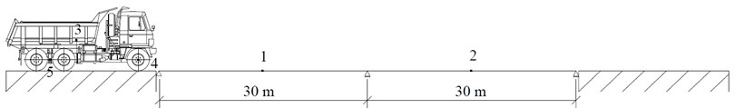
The bridge is a two-span continuous beam of the total length of 60 meters. The length of individual fields is 30 and 30 meters, Fig. 3. It is assumed the road profile with a smooth surface. The vehicle moves along the bridge with constant speed during the numerical simulation. In front of the bridge an area for acceleration the vehicle and behind the bridge an area for deceleration the vehicle is created. The acceleration and deceleration areas are modeled as rigid track.

For the purpose of comparing the results, a numerical simulation versus experiment, 5 points of interest were chosen. vehicle on a two-span bridge. These points are labeled from 1 to 5 in Fig. 3. Point (1) represents the middle of the 1st bridge span, point (2) the middle of the 2nd bridge span, point (3) the vehicle gravity center, point (4) the vehicle front axle and point (5) the vehicle rear axle.

Fig. 3Schematic outline of the modeled area

The vehicle arrives on the bridge already vibrated. Initial conditions on the vehicle and the bridge when the vehicle enters the bridge are given in Chapter 5.

The bridge model based on classical dynamics was solved in the environment of the program system MATLAB [16]. A custom program has been created to solve the task. To solve the equations of motion, the procedure od45 was used. It integrates the system of differential equations $y^{\text{'}}=f\left(t,y\right)$ from $t_0$ to $t_f$ with initial conditions $y_0$. For this reason, second-order equations of motion must be transformed into first-order equations by appropriate substitution. Ode45 is based on explicit Runge-Kutta Eqs. (4, 5), the Dormand-Prince pair. It is a one-step solver – in computing $y\left(t_n\right)$, it needs only the solution at the immediately preceding time point, $y\left(t_{n-1}\right)$. The output of the solution is done with a time step of 0.001 s.

The bridge model based on the finite element method was solved in the environment of the program system ADINA [13]. The Newmark’s method is used for the solution of equations of motion. The Newmark's method is an implicit method and is based on the integration of the differential equation after certain time steps $∆t$ at the time interval $t$, $t_{max}$. Time discretization is increasing for geometric discretization, and our unknowns are functional values at certain geometric and time points. Based on this, we can easily apply the procedures and algorithms used in static analysis of FEM. Basic relationships are based on the following assumptions:

Parameters $\alpha$ and $\beta$ has an influence on the stability of the solution. The method of linear acceleration is obtained by these coefficients with values $\alpha =$ 1/2 and $\beta =$ 1/6. Then we express the vectors and substitute equation at time $t+\mathrm{\Delta }t$:

and then:

where $\left[\widehat{K}\right]$ is a matrix of modified stiffness and $\left\{{\widehat{F}}_{t+∆t}\right\}$ is a vector of the modified load. From this, we can determine the displacements at nodal points at time $t+∆t$. The output of the solution is done with a time step of 0.001 s.

7. Results of numerical simulation

7.1. Influence of speed of vehicle motion

Put simply, the dynamics is about the mutual relationship between natural and excitation frequencies in a given dynamic system. The values of natural and excitation frequencies are influenced by many different factors – system parameters. Of all these factors, the impact of vehicle speed has a specific position, since it is meaningful to talk about the effect of all other parameters only in relation to specific vehicle speed. We are interested in the dynamic deflections of the bridge depending on the speed of the vehicle. The dependence of the maximum dynamic displacement in the middle of the bridge span $v_{max}$ on the vehicle speed $V$ is not a smooth curve. It contains a large number of local maxima and spikes. The character of function $v_{max}\left(V\right)$ is closely related to the discontinuous course of function $x\left(V\right)$ indicating, depending on the speed of the vehicle, the position of the vehicle on the bridge when the maximum deflection $v_{max}$ occurs. The position of the spikes in the $v_{max}\left(V\right)$ function corresponds to the discontinuity points (jumps) of the $x\left(V\right)$ function. The nature of the functional dependence $v_{max}\left(V\right)$ depends on the relationship between the basic natural frequency of the vehicle and the bridge. It has a rising tendency for real cases [6].

Use the symbols $v_{max,\mathrm{1,1}}$and$w_{max,\mathrm{1,1}}$ for maximum dynamic displacements in the middle of the 1st bridge span at the moments when the vehicle moves along the 1st span at classical and FEM computational models respectively. For the computational model of the bridge based on classical dynamics the values $v_{max,\mathrm{1,1}}$ were calculated in the interval of speed 5-130 km/h with the step 1 km/h. For the computational model of the bridge based on the finite element method, the values $w_{max,\mathrm{1,1}}$ were calculated in the interval of speed 5-130 km/h with the step 5 km/h. The mutual comparison of calculated values $v_{max,\mathrm{1,1}}$ and $w_{max,\mathrm{1,1}}$ as the functions of the vehicle speed are shown in Fig. 4.

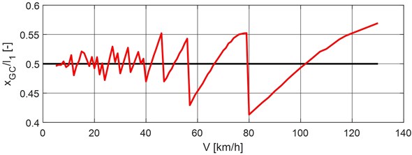
Dimensionless position of vehicle gravity center $x_{GC}/l_1$, when the maximum deflection $v_{max,\mathrm{1,1}}$occurs, as a function of the vehicle speed, is shown in Fig. 5.

Fig. 4Maximal deflections vmax, 1,1andwmax, 1,1 versus vehicle speed for classical and FEM bridge model

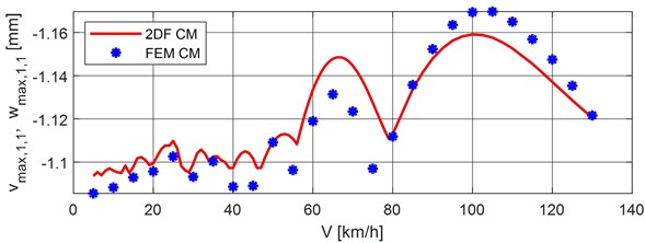
Fig. 5Dimensionless position of vehicle gravity center versus vehicle speed

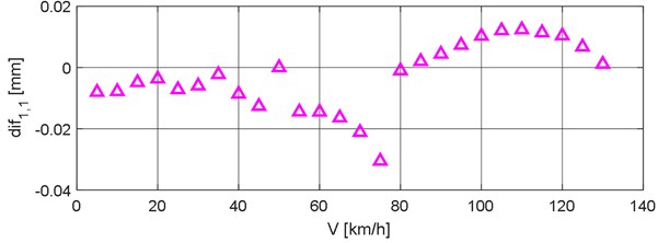
Comparing the maximum dynamic displacements, Fig. 4, it can be seen that both computational models of the bridge give comparable results. The differences in the dynamic displacements calculated for both bridge computational models are shown in Fig. 6. It can be seen in Fig. 6 that at the speed range of 1-80 km/h, the FEM model gives smaller displacement values than the classical model. Conversely, at the speed range of 80-130 km/h, the FEM computational model gives greater values of displacements than the classical model. The maximum negative difference of –0.0305 mm is at the speed of 75 km/h, the maximum positive difference of +0.0124 is at the speed of 110 km/h. At the speed 50 km/h, the difference is zero.

Fig. 6Differences of dynamic displacements, 2DF CM minus FEM CM, versus vehicle speed

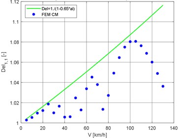
Given the nature of the $v_{max,\mathrm{1,1}}\left(V\right)$and$w_{max,\mathrm{1,1}}\left(V\right)$ curves, it would be appropriate to approximate the values of the maximal dynamic displacements by some envelope curve. In this case, it is preferable to work with dimensionless quantities. Let us define the value of the dynamic coefficient $\delta$ as the ratio of the maximum dynamic bridge deflection $w_{max,\mathrm{1,1}}$and the static deflection $w_s$:

14

${\delta }_{\mathrm{1,1}}=\frac{w_{max,\mathrm{1,1}}}{w_s}.$

The envelope curve equation of the dynamic coefficients may, for example, have the form:

15

${\delta }_{env}=\frac{1}{1-0.65\bullet \alpha }.$

The dimensionless coefficient $\alpha$, expressing the influence of the vehicle speed, is given by the relation:

16

$\propto =\frac{T_{\left(1\right)}}{{2T}_p},$

where $T_{\left(1\right)}$ is the period of bridge vibration in the first natural mode and $T_p$ is the time of crossing the bridge field [20]. The approximation of the dynamic coefficients $\delta$ by the envelope curve ${\delta }_{env}$ for the FEM computational model is shown in Fig. 7.

Fig. 7Approximation of dynamic coefficient by the envelope curve

7.2. Bridge and vehicle response at vehicle speed 70 km/h

The subject of the numerical simulation is the movement of a vehicle on a two-span bridge. The results of the numerical simulation are analyzed in five points. These points are labeled from 1 to 5 in Fig. 3. Point (1) represents the middle of the 1st bridge span, point (2) the middle of the 2nd bridge span, point (3) the vehicle gravity center, point (4) the vehicle front axle and point (5) the vehicle rear axle. The obtained results in these 5 points of interest are presented in Figs. 8-12 as the vertical deflections corresponding to a vehicle speed of 70 km/h for both classical and FEM computational models. This passage speed was chosen because it is the normal average speed at which heavy vehicles ride along road and bridge objects.

Dimensionless position of vehicle gravity center $x_{GC}/l_1$, when the maximum deflection $v_{max,\mathrm{1,1}}$occurs, as a function of the vehicle speed, is shown in Fig. 5.

Fig. 8Vertical deflection in the middle of the 1st bridge span, point nr. 1

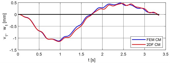
Fig. 9Vertical deflection in the middle of the 2nd bridge span, point nr. 2

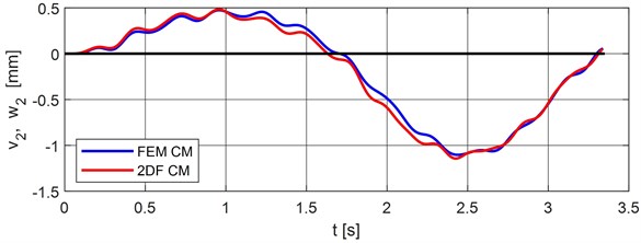
Fig. 10Vertical deflection of the vehicle center of gravity, point nr. 3

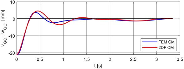
Fig. 11Vertical deflection of the vehicle front axle, point nr. 4

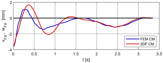
Fig. 12Vertical deflection of the vehicle rear axle, point nr. 5

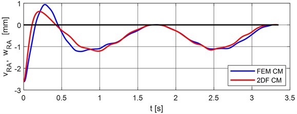
Comparison of maximal values of vertical deflections for classical and FEM calculation models are put into Table 1. The differences FEM model minus the classical model are put into Table 2.

Table 1Comparison of maximal vertical dynamic deflections of characteristic points of bridge and vehicle

	Classical model		FEM model
	Deflection [mm]	Time [s]	Deflection [mm]	Time [s]
–$v_1$, –$w_1$	–1.144642	0.967704	–1.123450	0.960000
+$v_1$, +$w_1$	+0.462120	2.464058	+0.479965	2.420000
+$v_2$, +$w_2$	+0.483276	0.955000	+0.474085	0.960000
–$v_2$, –$w_2$	–1.142974	2.428046	–1.103050	2.440000
$v_{GC}$, $w_{GC}$	+4.588611	0.452968	+3.772000	0.400000
$v_{FA}$, $w_{FA}$	+1.660963	0.367578	+1.080999	0.250000
$v_{RA}$, $w_{RA}$	+0.619245	0.207143	+0.940000	0.280000

Table 2Differences FEM minus classical model of maximal vertical dynamic deflections of characteristic points of bridge and vehicle

	Differences FEM minus classical model
	Deflection [mm]	Deflection in % FEM	Time [s]	Time in % FEM
–$v_1$, –$w_1$	–0.021192	–1.8863	–0.007704	–0.8025
+$v_1$, +$w_1$	+0.017845	+3.7180	–0.044058	–1.8206
+$v_2$, +$w_2$	–0.009191	–1.9387	+0.005000	+0.5208
–$v_2$, –$w_2$	–0.039924	–3.6194	+0.011954	+0.4899
$v_{GC}$, $w_{GC}$	–0.816611	–21.6493	–0.052968	–13.2420
$v_{FA}$, $w_{FA}$	–0.579964	–53.6507	–0.117578	–47.0312
$v_{RA}$, $w_{RA}$	+0.320755	+34.1229	+0.072857	+26.0204

8. Experimental validation

To verify the rightness of assumptions adopted in the design of the bridge model in the spirit of classical dynamics, the model experimental tests in laboratory conditions were carried out. The bridge model was designed as a steel two-span continuous beam with a constant cross-section [21]. The spans are $l_1=l_2=$ 1.45 m and the cross-section dimensions are 12×18 mm. Special equipment providing the movement of the load was developed, Fig. 13. In front of the beam the speeding-up path and behind the beam the braking path was built up.

Vertical deflections in the middle of the spans were measured by an inductive sensor IVR 99427, Fig. 14. Border and intermediate supports are illustrated in Fig. 14. The accelerometer BK 4508 was fitted at the beginning of the beam and at the beginning of the braking path.

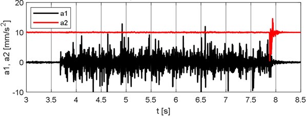
By comparing the records of these accelerometers, it is possible to determine the load passing time along the beam, Fig. 15. Load passing time $t_p$ is determined as the difference between the end time $t_e$ and the start time $t_s$ of the passage, $t_p=t_e–t_s$. The average speed of the movable load is determined as the ratio of the beam length and the passage time, $\stackrel{-}{e}=l_b/t_p$.

Fig. 13Towing unit with moving load and speeding-up path

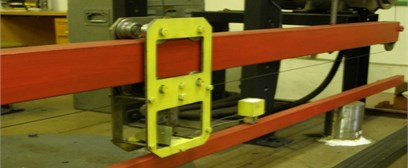
Fig. 14Inductive sensor IVR 99427 – border support and accelerometer BK 4508 – intermediate support

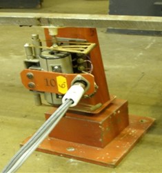
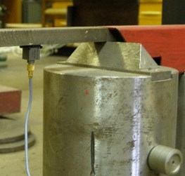
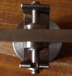
Fig. 15Records of accelerometers for determining the load passing time

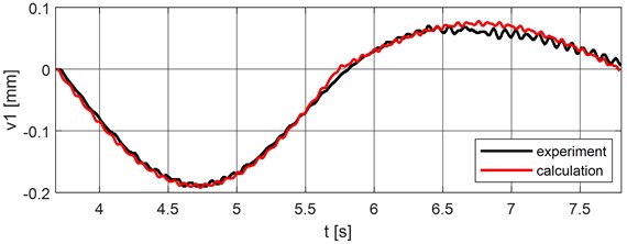
The mass of the moving load was $m_v=$ 220 g. Vertical deflections in the middle of the span were measured at different speeds of the moving load. The same processes were simulated numerically in MATLAB. Comparison of experimentally and numerically obtained records, at the speed of the moving load $\stackrel{-}{e}=$ 0.70731 m/s, is in Fig. 16.

Fig. 16Comparison of experimentally and numerically obtained results

9. Conclusions

Moving load effect on bridges is an important task solving in many workplaces in the world. The task can be solved numerically and experimentally. In the present time, numerical modeling of the problems of moving load effect on bridges is an effective tool for the solution of real tasks of engineering practice. To solve this problem it is possible to create various computational models. Models can be planar or spatial. They can be created in the spirit of classical dynamics or in the spirit of the finite element method. The models can be discrete with finite degrees of freedom, or the model parameters can be continually distributed. Discrete computational models are more advantageous from the point of view of the mathematical solution because the equations of motion have the form of ordinary differential equations.

The innovative contribution in solving vehicle-bridge interaction is modeling of the vehicles in combination with mass objects, damping and stiffness elements, which can better describe the real vehicle and its movement over the bridge construction.

The results of numerical studies show that even simple bridge models can give good results in certain areas. For example, the computational model of a bridge as a continuous beam with 2 degrees of freedom gives comparable results to the FEM model. The differences in deflections in the middle of individual fields range from 1 % to 4 %.

In engineering practice, the need for numerical modeling is very important. A large amount of data can be obtained using a properly functioning numerical model. This data is very important because in the past, it was possible to obtain this data only by means of a dynamic load test. These experimental in situ measurements are time-consuming and very expensive.

The quality of the input data determines the quality of the output results. Today, the level of computing technology is such high that all tasks can be solved in real-time. In practice, the engineer is interested in how the change of individual vehicle and bridge parameters influences the overall result of the solution. The results obtained by numerical analysis can be used differently. The primary interest is the optimal design of the bridge with regard to its durability and reliability [20].

A physical model in labo was created to verify the results obtained from numerical modeling. The results obtained in experimental measurements proved the correctness of the principle of the numerical model. The experiment is important in mechanics as it is the only way to verify numerically obtained results. Using the experiment, it is possible to verify the correctness of assumptions received in the creation of the computational model and also the numerical accuracy. For example, the results presented in Chapter 8 confirm that the assumptions used to create a discrete computational model in the spirit of classical dynamics were correct.