Identification of the parameters of a composite material by experimental-computational damping research

Eremin, V. P.; Guseva, E. E.; Bolshikh, A. A.

doi:10.21595/jve.2022.22670

Journal of Vibroengineering

Browse Journal

Submit article

Published: 14 February 2023

Check for updates

Identification of the parameters of a composite material by experimental-computational damping research

V. P. Eremin¹

E. E. Guseva²

A. A. Bolshikh³

^{1, 2, 3}Aircraft Design and Certification Department, Moscow Aviation Institute (National Research University), Moscow, Russia

Corresponding Author:

A. A. Bolshikh

Cite the article Download PDF

Downloads 276

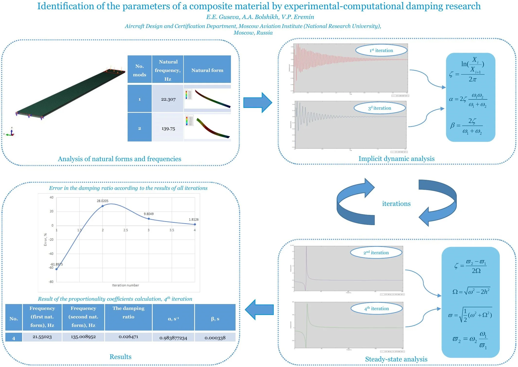
Abstract

Calculation of the modal and damping characteristics necessary to eliminate resonant oscillation of products made of polymeric materials requires reliable data on the elastic characteristics of the material. The problem is that the mechanical properties of polymer composite materials depend on a large number of factors. The aim of the work is to determine the damping coefficients for a layered composite material and the subsequent validation of the mathematical model. The Rayleigh damping model was chosen to calculate the damping coefficients. The choice is due to the fact that the resulting stiffness and mass matrix is determined by the natural oscillation modes of the problem without attenuation, which makes it possible to split the modes into separate dynamic subtasks. A sample made according to the ASTM standard was chosen as the object of study. To increase an error of the calculation, the mathematical model of the sample was modeled in detail by the finite element method using the technique of layer-by-layer modeling. The method for determining the damping coefficients is carried out in three stages. At the first stage, with the help of modal analysis, the natural oscillation modes are determined, corresponding to the nature of the oscillation studied in the experiment. At the second stage, an implicit dynamic analysis with default damping parameters in order to calculate the damping ratio is performed. At the last stage, a steady-state dynamic analysis taking into account the characteristics obtained in the previous stages. Next, an iterative process begins, including implicit and steady-state dynamic analyses, performed alternately. At each step, the previously calculated Rayleigh proportionality coefficients are introduced into the model. As a result of the identification of the mathematical model, the damping coefficients $α$ and $β$ are calculated. The damping experiment was chosen as a validation problem. The damping ratio $ζ$ was chosen as the criterion of convergence with the experimental data.

Identification of the parameters of a composite material by experimental-computational damping research

Highlights

Tests of composite materials for damping properties (the damping ratio and proportional coefficients) are modeled in accordance with Rayleigh theory. The finite element method is used for modeling.
The damping properties of a layered composite material are calculated. The methodology includes the results of frequency analysis, dynamic implicit analysis and dynamic stationary state analysis.
The damping properties are refined iteratively up to an error of 1.81% relative to the experimental data.

1. Introduction

Polymer composite materials (PCM), in particular carbon plastics, are widely used for the manufacture of loaded parts of aircraft and aircraft engines due to the possibility of lightweight construction without reducing strength [1-4]. It is known, for example, that the use of PCM in the design of the airframe of Boeing 787 aircraft reaches 50 % by weight [2, 4]. The wide use of PCM is envisaged in the creation of domestic aircraft and aircraft engines of new generation [2, 3].

The problem of search of natural frequencies can be solved with and without damping. Most often the presence of damping in the system affect not only natural frequencies, but also the natural forms. If the excitation frequency is close to the natural frequency (e.g. in the ±50 % band), consideration of damping is very important, as can be seen from the resonant response curves. In this case, attention must be paid to the selection of suitable and correct damping criteria values. Near resonant, the response is almost completely dependent on the damping value, so, for example, changing the hysteresis loss factor from 0.01 to 0.02 could end up doubling the estimated stress level [8].

In time-domain dynamic studies, damping usually has little effect on the final results. Exceptions are encountered when modeling wave propagation or loads that excite some of the resonant frequencies of a structure [9].

On the other hand, setting the damping in the time domain analysis allows us to stabilize the temporal computational scheme. Parasitic waves often appear in designs that are not interesting for the main analysis. If they are not quenched, the time step can become excessively small. To extinguish the parasitic waves, one can add losses at high frequencies to the model [10-11].

Rayleigh damping is a simple approach to forming a damping matrix as a linear combination of a mass matrix and a stiffness matrix. The Rayleigh damping model makes it possible to calculate the proportionality coefficients depending on the oscillation frequencies, which, in turn, makes it possible to perform calculations for the oscillation forms in different directions. This approach is very useful in the study of composite materials, since in this way, by changing the studied frequencies, it is possible to obtain proportionality coefficients in different directions and take into account the anisotropy of properties.

This damping model is clearly not related to any physical loss mechanisms. Initially this model was used because such a resulting matrix is diagonalized by the natural forms of the problem without damping, which allows us to break the modes into separate dynamic subproblems.

In [12], the author investigates the possibility of polymer sample identification using modal analysis and validates the mathematical model with the tests performed. The maximum error with the experiment is 3.9 %, which indicates the correctness of the chosen method. However, the author does not consider the friction between the layers in the mathematical model and this modeling method is not suitable for determining the damping characteristics.

In this work, the model of the sample was made in layers. The damping characteristics are determined by an iterative method, including modal, implicit dynamic and steady-state analyses performed using the finite element method. Comparison with the experiment is carried out using the damping ratio. The resulting error at the last iteration is 1.81 %.

2. Analysis of natural forms and frequencies

2.1. Model description

Glass Laminate Aluminum Reinforced Epoxy (GLARE) was chosen as the test specimen. The sample is a structural layered hybrid material consisting of thin (0.3-0.4 mm) sheets of aluminum alloys (Al-Li medium strength reduced density alloy) and interlayers of fiberglass. Plastic layers usually consist of several monolayers of unidirectional adhesive prepreg reinforced with high-strength glass fillers. Parameters of the materials are given in Table 1.

Thicknesses of the sample layers are shown in Table 2.

Table 1Mechanical properties of materials

Material	Orientation	Elastic modulus $E$ , MPa	Poisson’s ratio $η$	Density $ρ$ , t/mm³
1441 alloy sheet	–	79000	0.33	2.6E-9
Fiberglass	0°	50000	0.3	1.78E-9
Fiberglass	90°	12000	0.07	1.78E-9

Table 2Thicknesses of the sample layers

Material	Thickness, mm
1441 alloy sheet 0	0.35
Fiberglass 0°	0.3
1441 alloy sheet 0	0.35
Fiberglass 90°	0.3
1441 alloy sheet 0	0.35

The geometric characteristics of the sample conform are shown in Table 3.

Table 3Geometric parameters of the sample

Sample	Length, mm	Width, mm	Thickness, mm
GLARE	255	20	1.65

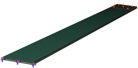
The finite-element model consists of 25000 elements of order 1 HEXA type (three-dimensional hexagonal volume element with eight nodes and three rotational degrees of freedom). In order to refine the results of the finite element analysis, the sample is made by layer-by-layer modeling. The model of the sample is shown in Fig. 1.

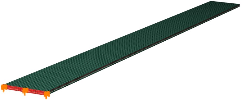
The natural forms were calculated by the Lanczos block method with spectral transformations [14]. The model is bounded at the end by all degrees of freedom, as shown in Fig. 2. The constraint is chosen according to the experimental conditions.

Fig. 1General view of the FEM

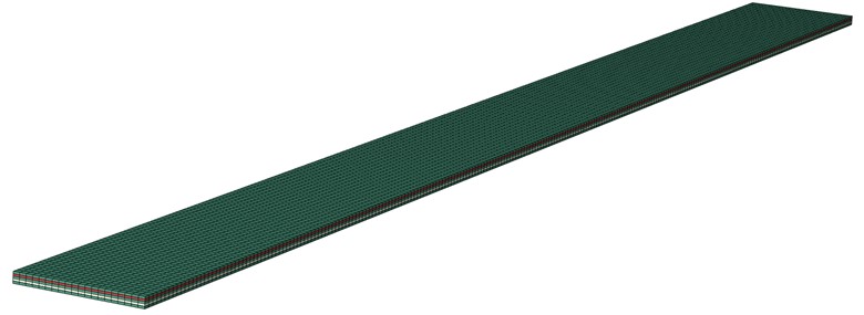
Fig. 2Boundary conditions for modal analysis

2.2. Calculation of natural forms and frequencies

At the first step, a modal analysis is performed, as a result of which the first two bending natural frequencies and forms were determined. The obtained data are presented in Table 4.

Results of calculation of the natural frequencies by the experimental method and the finite element method are summarized in Table 5.

As can be seen from the table, the damping ratio turned out to be an order of magnitude higher than the damping ratio obtained experimentally, which indicates the need to refine the material model. For this purpose, proportionality coefficients are introduced into the material properties. The calculation of the coefficients was carried out by the iterative method described in detail in Chapter (3.2). As a result of the measures described above, the values presented in Table 6 were obtained.

Table 4The result of the modal analysis

No. mods	Natural frequency, Hz	Natural form
1	22.307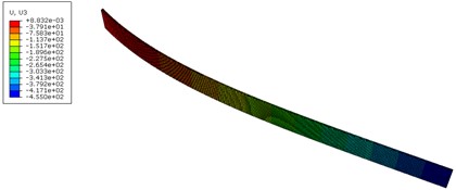
2	139.75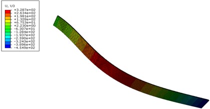

Table 5Comparison of experimental data with initial data obtained by FEM

Method	First natural frequency, Hz	Error, %
Experiment	21.5	3.75
FEM	22.307	3.75

Table 6Comparison of experimental data with refined data obtained by FEM

Method	First natural frequency, Hz	Error, %
Experiment	21.5	0.23
FEM	21.55023	0.23

3. Implicit dynamic analysis

3.1. Model description

In order to perform a nonlinear implicit dynamic analysis, an initial displacement was applied to the finite-element model to create excitation. The boundary conditions at the first calculation step are shown in Fig. 3. In the second step, the load applied in the first step is removed and the specimen moves freely. In order to obtain a detailed picture of the specimen oscillation, the removal time was chosen to be 0.01 s. Total force applied to the sample was 10 N. A similar analysis was carried out without considering material damping and with time integrator parameter (TIP) –0.05 included. The methodology for determining the damping properties is described below. The damping ratio $ζ$ was chosen as the convergence criterion.

Fig. 3Loading conditions for implicit dynamic analysis

3.2. Description of the calculation methodology

To model the damping properties of the material, the Rayleigh proportional damping model, is used:

1

C = α M + β K,

where $C$ – global damping matrix, $M$ – global mass matrix, $K$ – global stiffness matrix, $α$ – coefficient characterizing the inertial damping, $β$ – coefficient characterizing the structural damping.

The damping coefficient of oscillation can be found through the natural frequencies:

2

ζ_{i} = \frac{α}{2 ω_{i}} + \frac{β ω_{i}}{2},

where $ζ_{i}$ – the damping ratio, $α$ – coefficient characterizing the inertial damping, $ω_{i}$ – natural frequencies of the sample, $β$ – coefficient characterizing the structural damping.

The main advantage of this method is that it simulates the damping parameters for a material rather than for a particular structure, i.e. by determining the damping parameters for a given sample, it is possible to use this model to calculate other structures made of this material.

To calculate the proportionality coefficients $α$ and $β$ it is necessary to carry out a modal calculation to determine the natural frequencies of the sample, corresponding to two successive bending forms of oscillation.

After determining the necessary oscillation frequencies, a calculation similar to the tests for the form at the frequency corresponding to the bending oscillation is performed. The calculation is carried out within the framework of the general nonlinear dynamic analysis using implicit time integration. The result is the time-dependence of specimen displacement, from which the amplitudes of the first and second free bending oscillation of the specimen are determined. Then, according to the formula given below, the damping ratio is determined [15-18]:

3

ζ = \frac{l n (\frac{X_{i}}{X_{i + 1}})}{2 π},

where $ζ$ – the damping ratio, $X_{i}$ – amplitude of the ( $i$ ) free oscillation, $X_{i + 1}$ – amplitude of the ( $i + 1$ ) free oscillation.

The oscillation frequencies were calculated using a well-known formula:

4

ϖ = \frac{1}{T},

where $ϖ$ – free oscillation frequency, $T$ – time period.

Proportionality coefficients $α$ and $β$ could be calculated by the following equations [20]:

5

α = 2 ζ \frac{ω_{1} ω_{2}}{ω_{1} + ω_{2}},

where $α$ – proportionality factor, determining the damping parameters at low frequencies, $ζ$ – the damping ratio, $ω_{1}$ – the first natural frequency, $ω_{2}$ – the second natural frequency:

6

β = \frac{2 ζ}{ω_{1} + ω_{2}},

where $β$ – proportionality coefficient, determining the damping parameters at high frequencies, $ζ$ – the damping ratio, $ω_{1}$ – the first natural frequency, $ω_{2}$ – the second natural frequency.

The data obtained should be clarified due to the fact that, first, modal analysis does not consider the damping properties of the material, therefore, the obtained values of natural frequencies are overestimated; second, in the dynamic calculation the damping of oscillation is due to the general kinematic energy dissipation of the system, but not the damping properties of the material.

4. Steady-state analysis

4.1. Model description

After the initial calculation of the proportionality coefficients, a dynamic analysis of the stationary state based on the natural forms and frequencies is performed, which is used to calculate the response of the system to harmonic excitation. Steady-state linear dynamic analysis uses the set of natural forms extracted in a previous modal step to calculate the steady-state solution as a function of the frequency of the applied excitation. To conduct the steady-state analysis, the same as in implicit analysis boundary and loading conditions shown in Fig. 3 were used. The frequency range was selected from 0 to 200 Hz.

Based on the results obtained as a result of the calculation, the natural frequencies and amplitudes of oscillation are specified. The damping ratio $ζ$ and proportionality coefficients α and $β$ are recalculated again respectively.

4.2. Description of the calculation methodology

The test results were processed using the fast Fourier transform method to obtain the amplitude-frequency response (AFR) of the realized oscillation [22]. A peak corresponding to the first resonant frequency was determined on the obtained AFR. The width of the found peak allows us to determine the sample the damping ratio $ζ$ based on the following equation:

7

ζ = \frac{ϖ_{2} - ϖ_{1}}{2 Ω},

where $ζ$ – the damping ratio, $Ω$ – resonant frequency, $ϖ_{1} < ϖ_{2}$ – frequencies near resonant, at which the amplitude value decreases by a factor of √2 compared to the resonant amplitude.

To determine the damping ratio, the Eq. (7) was used. The peak shown on the graph corresponds to the resonant frequency. The following relation is carried out between the natural frequency and the resonant frequency:

8

Ω = \sqrt{ω^{2} - 2 h^{2}},

where $Ω$ – the resonant frequency, $ω$ – the natural frequency, $h$ – viscous damping parameter.

The frequency of free damped oscillation is determined by the formula:

9

ϖ = \sqrt{ω^{2} - h^{2}},

where $ϖ$ – the free oscillation frequency, $ω$ – the natural frequency, $h$ – viscous damping parameter.

From Eqs. (8, 9), knowing the resonant and natural frequency, the oscillation frequency can be expressed in the following way:

10

ϖ = \sqrt{\frac{1}{2} (ω^{2} + Ω^{2})},

where $ϖ$ – the free oscillation frequency, $ω$ – the natural frequency, $Ω$ – the resonant frequency.

To calculate the frequency of free damped oscillation corresponding to the second natural form, it is assumed that it decreases relative to the second natural frequency in proportion to the decrease in the frequency of oscillation in the first natural form:

11

ϖ_{2} = ω_{2} \frac{ω_{1}}{ϖ_{1}},

where $ϖ_{2}$ – free oscillation frequency corresponded to the second natural form, $ω_{2}$ – the second natural frequency, $ϖ_{1}$ – free oscillation frequency corresponded to the first natural form, $ω_{1}$ – the first natural frequency.

Then the proportionality coefficients are calculated using the Eqs. (5, 6). To calculate the proportionality coefficients, the natural frequencies $ω$ in the Eqs. (5, 6) were replaced by the frequencies of free damped oscillation $ϖ$ .

5. Results

This section presents data and graphs for all iterations performed.

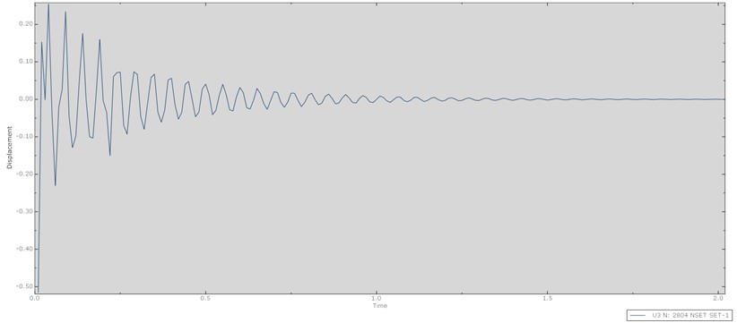
As described above, the first step is dynamic implicit analysis with a built-in damping parameter. The graphs and the numerical data obtained at iteration No. 1 are shown in Fig. 4 and in Table 7.

Fig. 4The result of the implicit dynamic analysis, first iteration

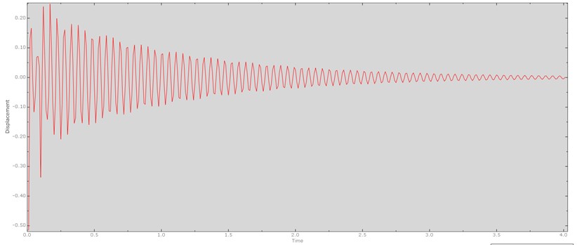
In the above graph, displacement is expressed in millimeters (mm), time is expressed in seconds (s). The damping ratio and frequency were calculated for all peaks of oscillation on the graph, then the values were averaged.

Hereinafter, the symbol “No.” refers to the number of iterations at which the values were obtained.

Table 7Result of the proportionality coefficients calculation, first iteration

No.	First natural frequency, Hz	Second natural frequency, Hz	The damping ratio	$α$ , s^-1	$β$ , s
1	22.307	139.75	0.009907	0.381138	0.000122

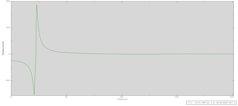
Then a dynamic analysis of the stationary state was carried out. The graphs and the numerical data obtained at iteration No. 2 are shown in Fig. 5 and in Table 8.

Fig. 5The result of the dynamic analysis of the stationary state based on natural forms and natural frequencies (second iteration)

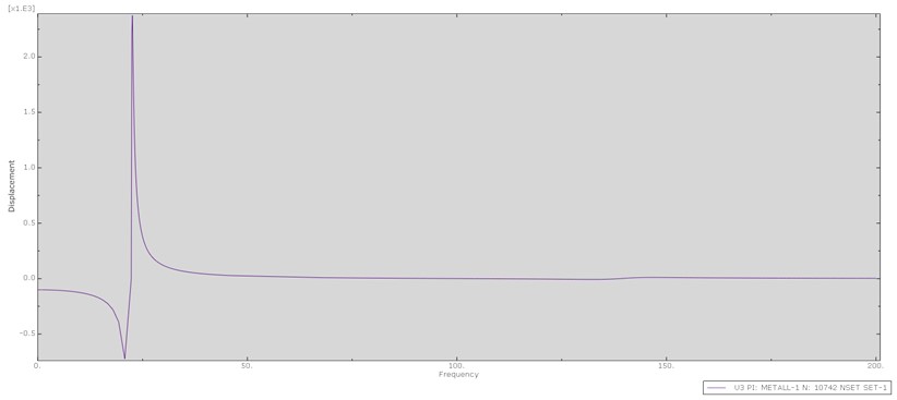
In the above graph, displacement is expressed in millimeters (mm), frequency is expressed in hertz (Hz).

Displacements in this type of analysis do not make physical sense; mathematically, the amplitude at resonance tends to infinity. In this case, the displacements are used only to determine the parameters of the resonant peak.

Table 8Result of the proportionality coefficients calculation, second iteration

No.	Frequency (first nat. form), Hz	Frequency (second nat. form), Hz	The damping ratio	$α$ , s^-1	$β$ , s
1	21.55023	135.008952	0.033285	1.237140	0.000425

In the following iterations, the set of implicit and dynamic analysis of the stationary state was used again and the results were processed. The number of approximations is chosen from the condition of sufficiency to determine the character of the dynamics of the iteration process.

Then an implicit dynamic analysis was carried out. The graphs and the numerical data obtained at iteration No. 3 are shown in Fig. 6 and in Table 9.

Fig. 6The result of the implicit dynamic analysis, third iteration

In the above graph, displacement is expressed in millimeters (mm), time is expressed in seconds (s). The damping ratio and free oscillation frequency was calculated for all peaks of oscillation on the graph, then the values were averaged.

Table 9Result of the proportionality coefficients calculation, third iteration

No.	Frequency (first nat. form), Hz	Frequency (second nat. form), Hz	The damping ratio	$α$ , s^-1	$β$ , s
3	19.5977	122.77665	0.028549	0.9649711	0.000401

Then a dynamic analysis of the stationary state was carried out. The graphs and the numerical data obtained at iteration No. 4 are shown in Fig. 7 and in Table 10.

Fig. 7The result of the dynamic analysis of the stationary state based on natural forms and natural frequencies (fourth iteration)

In the above graph, the displacement is expressed in millimeters (mm), frequency is expressed in hertz (Hz).

Table 10Result of the proportionality coefficients calculation, fourth iteration

No.	Frequency (first nat. form), Hz	Frequency (second nat. form), Hz	The damping ratio	$α$ , s^-1	$β$ , s
4	21.55023	135.008952	0.026471	0.983877234	0.000338

To describe the nature of the dynamics of the iteration process the graph of dependence of the error of calculation of the damping coefficient on the number of iteration. It is shown in Fig. 8.

Fig. 8Error in the damping ratio according to the results of all iterations

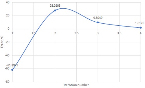
As can be seen from the graphs, the error of the damping ratio takes its minimum value on the fourth iteration. A leap in the graph at the second iteration is associated with the replacement of the damping model proposed by the program with the Rayleigh damping model, whose data is entered manually.

6. Experiment description

The experiment data was taken from the article [22]. The paper considers the tests of several samples of GLARE, as well as tests of sandwich beam.

Dynamic tests of GLARE samples were carried out using the method of free damped oscillation. In the tests, the samples were rigidly fixed with a clamp at one end, and loading conditions were set at the other end, leading to the occurrence of damped bending oscillation, mainly according to the first natural form. The length of the fixed part of the GLARE samples was 15 mm (not included in the total length of the sample in the model, which is 255 mm). To excite oscillation, the free end of the fixed sample was either struck with a metal striker, or its initial deviation from the equilibrium position with a maximum deflection of 5-15 mm was set. Both loading options (static – by impact and kinematic – by drawing the end of the sample) led to the same measurement results, with a difference not exceeding the error of the measuring equipment. To register the amplitude of free damped oscillation of the samples, a video recording was carried out. The tests used a VideoSprint-G4 video camera with a shooting frequency of 800 cad/s. The test results were processed using the fast Fourier transform method to obtain the amplitude-frequency response (AFR) of the realized oscillation [22].

7. Conclusions

As a result of this work the methodology of calculation of damping properties for the composite material was developed. The technique is based on the modal analysis of the material sample and qualified by the results of the experiment.

Mathematical models have been developed to carry out oscillation virtual tests. The layer-by-layer modeling technique used to build the model showed high error of the results and can be used not only for model identification, but also for strength tests of the specimen to determine the character of fracture.

In the future, it is planned to apply the developed method for structurally similar samples. Calculations according to the presented methodology can be carried out for the forms of oscillation in different directions and thus obtain damping coefficients in different directions, which will allow one to create a complete model of the damping of the composite material. The model can be improved by introducing cohesive layers to account for the matrix.

The combined method of calculating $α$ and $β$ coefficients to calculate damping according to Rayleigh’s model can be applied at the design stage of aircraft structures products and thus obtain refined results of static and dynamic strength by identifying the model.

References

G. Wu and J.-M. Yang, “The mechanical behavior of GLARE laminates for aircraft structures,” Journal of The Minerals, Metals and Materials Society, Vol. 57, No. 1, pp. 72–79, Jan. 2005, https://doi.org/10.1007/s11837-005-0067-4

Publisher
L. B. Vogelesang and A. Vlot, “Development of fibre metal laminates for advanced aerospace structures,” Journal of Materials Processing Technology, Vol. 103, No. 1, pp. 1–5, Jun. 2000, https://doi.org/10.1016/s0924-0136(00)00411-8

Publisher
V. V. Antipov, N. Yu. Serebrennikova, O. G. Senatorova, L. V. Morozova, N. F. Lukina, and Yu. N. Nefedova, “Hybrid layered materials with a low rate of fatigue crack development,” Vestnik Mashinostroeniya, Vol. 61, No. 12, pp. 45–49, 2016.

Search CrossRef
V. V. Shestov, V. V. Antipov, N. Yu. Serebrennikova, and Yu. N. Nefedova, “High-strength layered material based on aluminum-lithium alloy sheets,” Technology of Light Alloys, Vol. 53, No. 1, pp. 119–123, 2016.

Search CrossRef
Z. Ming, P. A. Mbango-Ngoma, D. Xiao-Zhen, and C. Qing-Guang, “Numerical investigation of the trailing edge shape on the added damping of a Kaplan turbine runner,” Mathematical Problems in Engineering, Vol. 2021, pp. 1–11, Aug. 2021, https://doi.org/10.1155/2021/9559454

Publisher
M. Salehi, P. Sideris, and A. B. Liel, “Numerical simulation of hybrid sliding-rocking columns subjected to earthquake excitation,” Journal of Structural Engineering, Vol. 143, No. 11, p. 04017149, Nov. 2017, https://doi.org/10.1061/(asce)st.1943-541x.0001878

Publisher
W. Ma and X. Liu, “Phased microphone array for sound source localization with deep learning,” Aerospace Systems, Vol. 2, No. 2, pp. 71–81, Dec. 2019, https://doi.org/10.1007/s42401-019-00026-w

Publisher
C. Jagels, L. Reichel, and T. Tang, “Generalized averaged Szegő quadrature rules,” Journal of Computational and Applied Mathematics, Vol. 311, pp. 645–654, Feb. 2017, https://doi.org/10.1016/j.cam.2016.08.038

Publisher
D. J. Ewins, Modal Testing: Theory, Рractice and Аpplication. Baldock: Research Studies Press LTD, 2000.

Search CrossRef
J. Duan and Z. Zhang, “An efficient method for nonlinear flutter of the flexible wing with a high aspect ratio,” Aerospace Systems, Vol. 1, No. 1, pp. 49–62, Jun. 2018, https://doi.org/10.1007/s42401-018-0009-9

Publisher
W. Heylen, S. Lammens, and P. Sas, Modal Analysis Theory and Testing. Leven: Katholieke Universiteit Leuven.

Search CrossRef
M. S. Nikhamkin, S. V. Semenov, and D. G. Solomonov, “Application of experimental modal analysis for identification of laminated carbon fiber-reinforced plastics model parameters,” in Proceedings of the 4th International Conference on Industrial Engineering, pp. 487–497, 2019, https://doi.org/10.1007/978-3-319-95630-5_51

Publisher
M. M. Kamel and Y. A. Amer, “Response of parametrically excited one degree of freedom system with non-linear damping and stiffness,” Physica Scripta, Vol. 66, No. 6, pp. 410–416, Jan. 2002, https://doi.org/10.1238/physica.regular.066a00410

Publisher
M. H. Gutknecht, “A completed theory of the unsymmetric Lanczos process and related algorithms, Part I,” SIAM Journal on Matrix Analysis and Applications, Vol. 13, No. 2, pp. 594–639, Apr. 1992, https://doi.org/10.1137/0613037

Publisher
D. L. Mcculloch et al., “ISCEV Standard for full-field clinical electroretinography (2015 update),” Documenta Ophthalmologica, Vol. 130, No. 1, pp. 1–12, Feb. 2015, https://doi.org/10.1007/s10633-014-9473-7

Publisher
E. Erduran, “Evaluation of Rayleigh damping and its influence on engineering demand parameter estimates,” Earthquake Engineering and Structural Dynamics, Vol. 41, No. 14, pp. 1905–1919, Nov. 2012, https://doi.org/10.1002/eqe.2164

Publisher
J. F. Hall, “Problems encountered from the use (or misuse) of Rayleigh damping,” Earthquake Engineering and Structural Dynamics, Vol. 35, No. 5, pp. 525–545, Apr. 2006, https://doi.org/10.1002/eqe.541

Publisher
P. Jehel, P. Léger, and A. Ibrahimbegovic, “Initial versus tangent stiffness-based Rayleigh damping in inelastic time history seismic analyses,” Earthquake Engineering and Structural Dynamics, Vol. 43, No. 3, pp. 467–484, Mar. 2014, https://doi.org/10.1002/eqe.2357

Publisher
M. Barabash, B. Pisarevskyi, and Y. Bashynskyi, “Material damping in dynamic analysis of structures (with LIRA-SAPR program),” Civil and Environmental Engineering, Vol. 16, No. 1, pp. 63–70, Jun. 2020, https://doi.org/10.2478/cee-2020-0007

Publisher
V. S. Geraschenko, A. S. Grishin, and N. I. Gartung, “Approaches for the calculation of Rayleigh damping coefficients for a time-history analysis,” SUSI 2018, Vol. 180, No. 11, pp. 227–237, Jun. 2018, https://doi.org/10.2495/susi180201

Publisher
S. Nikolaev, S. Voronov, and I. Kiselev, “Estimation of damping model correctness using experimental modal analysis,” Vibroengineering PROCEDIA, Vol. 3, pp. 50–54, Oct. 2014.

Search CrossRef
O. A. Prokudin, Y. O. Solyaev, A. V. Babaytsev, A. V. Artemyev, and M. A. Korobkov, “Dynamic characteristics of three-layer beams with load-bearing layers made of alumino-glass plastic,” PNRPU Mechanics Bulletin, No. 4, pp. 260–270, Dec. 2020, https://doi.org/10.15593/perm.mech/2020.4.22

Publisher

About this article

Received

29 April 2022

Accepted

17 October 2022

Published

14 February 2023

SUBJECTS

Mechanical vibrations and applications

DOI

https://doi.org/10.21595/jve.2022.22670

Keywords

Rayleigh damping model

natural frequencies

the damping ratio

finite element method

Acknowledgements

The article is prepared in the implementation of the program for the creation and development of the World-Class Research Center “Supersonic” for 2020-2025 funded by the Ministry of Science and Higher Education of the Russian Federation (Grant agreement of April 20, 2022 No. 075-15-2022-309).

Data Availability

The datasets generated during and/or analyzed during the current study are available from the corresponding author on reasonable request.

Conflict of interest

The authors declare that they have no conflict of interest.

This is an open access article distributed under the Creative Commons Attribution License, which permits unrestricted use, distribution, and reproduction in any medium, provided the original work is properly cited.

Next article in issue Next

Research article

2022 07 07

Measurement of natural frequency and mechanical damping of thin brass diaphragm by pulsed laser generated vibrations

Muhammad Sohail Azam, Azhar Hussain Malik, Afshan Irshad, Mazhar Iqbal, Izhar Ahmad

Research article

2020 03 23

Identification of non-proportional structural damping using experimental modal analysis data

Akın Oktav

Research article

2019 11 28

Free vibration analysis of simply supported rectangular plates

Ganesh Naik Guguloth, Baij Nath Singh, Vinayak Ranjan

Research article

2017 06 30

Modal parameter identification of a three-storey structure using frequency domain techniques FDD and EFDD and time domain technique SSI: experimental studies and simulations

Nader Mohammadi, Mehrdad Nasirshoaibi

V. P. Eremin, E. E. Guseva, and A. A. Bolshikh, “Identification of the parameters of a composite material by experimental-computational damping research,” Journal of Vibroengineering, Vol. 25, No. 3, pp. 456–467, Feb. 2023, https://doi.org/10.21595/jve.2022.22670

Copy Extrica

Copied to clipboard!

TY  - JOUR
DO  - 10.21595/jve.2022.22670
UR  - https://doi.org/10.21595/jve.2022.22670
TI  - Identification of the parameters of a composite material by experimental-computational damping research
T2  - Journal of Vibroengineering
AU  - Eremin, V. P.
AU  - Guseva, E. E.
AU  - Bolshikh, A. A.
PY  - 2023
DA  - 2023/02/14
PB  - JVE International Ltd.
SP  - 456-467
VL  - 25
IS  - 3
SN  - 1392-8716
SN  - 2538-8460
ER  - 

Copy Ris

Copied to clipboard!

@article{Eremin_2023,
	doi = {10.21595/jve.2022.22670},
	url = {https://doi.org/10.21595/jve.2022.22670},
	year = 2023,
	month = {feb},
	publisher = {{JVE} International Ltd.},
	volume = {25},
	number = {3},
	pages = {456--467},
	author = {V. P. Eremin and E. E. Guseva and A. A. Bolshikh},
	title = {Identification of the parameters of a composite material by experimental-computational damping research},
	journal = {Journal of Vibroengineering}
}

Copy Bibtex

Copied to clipboard!

[1]V. P. Eremin, E. E. Guseva, and A. A. Bolshikh, “Identification of the parameters of a composite material by experimental-computational damping research,” Journal of Vibroengineering, vol. 25, no. 3, pp. 456–467, Feb. 2023, doi: 10.21595/jve.2022.22670.

Copy IEEE

Copied to clipboard!

Eremin, V. P., E. E. Guseva, and A. A. Bolshikh. “Identification of the Parameters of a Composite Material by Experimental-Computational Damping Research.” Journal of Vibroengineering 25, no. 3 (February 14, 2023): 456–67. https://doi.org/10.21595/jve.2022.22670.

Copy Chicago

Copied to clipboard!

Identification of the parameters of a composite material by experimental-computational damping research

Abstract

Highlights

1. Introduction

2. Analysis of natural forms and frequencies

2.1. Model description

2.2. Calculation of natural forms and frequencies

3. Implicit dynamic analysis

3.1. Model description

3.2. Description of the calculation methodology

4. Steady-state analysis

4.1. Model description

4.2. Description of the calculation methodology

5. Results

6. Experiment description

7. Conclusions

References

About this article

Related Articles