Abstract
Mounting sensors in disk stack separators is often a major challenge due to the operating conditions. However, a process cannot be optimally monitored without sensors. Virtual sensors can be a solution to calculate the sought parameters from measurable values. We measured the vibrations of disk stack separators and applied machine learning (ML) to detect whether the separator contains only water or whether particles are also present. We combined seven ML classification algorithms with three feature engineering strategies and evaluated our model successfully on vibration data of an experimental disk stack separator. Our experimental results demonstrate that random forest in combination with manual feature engineering using domain specific knowledge about suitable features outperforms all other models with an accuracy of 91.27 %.
Highlights
- Vibration data was used successfully to determine if there is only water or in addition also yeast in a disk stack separator.
- Three different feature selection techniques were compared and seven machine learning algorithms were applied.
- The best performance was reached with random forest classifier and the manually selected features RMS and kurtosis.
1. Introduction
Condition monitoring carried out by analyzing vibration data helps to detect or anticipate any significant failure [1]. Especially in disk stack separators, where installing a sensor inside the separator is impossible due to rough operating conditions, alternative ways to monitor its status are needed. Vibration analysis is frequently carried out to detect bearing defects in a wide range of industrial machinery, including induction motors, centrifugal pumps, and wind turbines [2], [3], [4], [5]. Also, for disk stack separators, vibration data has been used before for fault detection [6]. So far, there are no studies which determine if particles are present inside a separator using ML algorithms and comparing different feature engineering strategies.
In our work, we analyzed data from vibration sensors mounted on the outside of a disk stack separator to determine whether it contains only water or in addition other raw particles such as yeast. Being able to classify its content, provides the basis for further analyses, such as the detection of fouling or disposals. We compared three different feature engineering strategies and used seven popular classification algorithms, which are: Naive Bayes (NB) [7], logistic regression (LR) [8], -nearest neighbors (KNN) [2], [5], support-vector machine (SVM) [7], [9], random forest (RF) [8], 1D convolutional neural network (1DCNN) [10], and artificial neural network (NN) [3], [9] which are widely used in the manufacturing industry for condition monitoring.
2. Experimental setup
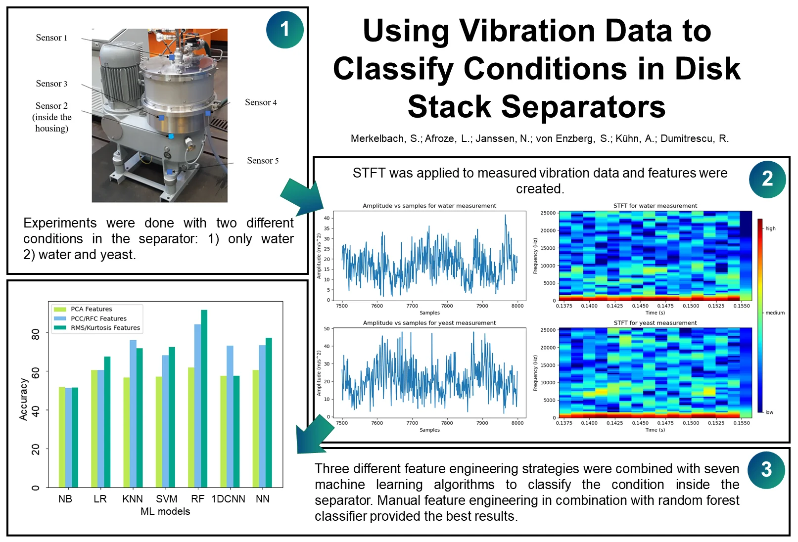
We carried out the experiments in a laboratory at the Chair of Fluid Mechanics of the University of Wuppertal using an experimental disk stack separator for liquid-solid separation with a belt drive. Five 3-axis acceleration sensors were placed on the separator, and their locations are shown in Fig. 1. A sampling frequency of 51,200 Hz and a period of 4 s were used for each measurement. Eleven different experiments were done where each had an average duration of 1 hour, resulting in 181 measurements. Among these eleven experiments, six were conducted only with water, and five were done with water and yeast particles.
Fig. 1Experimental separator with sensor locations which was used for the experiments in the laboratory at the Chair of Fluid Mechanics of the University of Wuppertal (GEA, 2022)
3. Data-driven modeling
3.1. Data Preparation
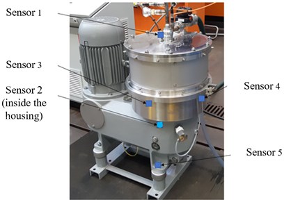
From the collected data, the spherical coordinates were calculated from the -, - and -directions of each of the five acceleration sensors. Short-time Fourier transform (STFT) was applied to the radial distance because it provides the amplitude of the vibration signal (see Fig. 2). In our case, STFT divides a period of 4 s into 6,400 equal-sized segments using the Hann window as window function and applies Fourier transform on each segment while considering FFT size as 64. This resulted in a total number of 181×64 = 11,584 distinct data points for the five sensors, of which 5,952 were labeled as water and 5,632 as yeast. As an example, the STFT of a small amount of data points is shown in Fig. 2 at the right side. A clear difference between water (top) and yeast (down) can be seen in the diagram. With appropriate feature engineering, this difference can be increased.
Fig. 2Amplitude (left) and STFT (right) for water (top) and yeast (down)
3.2. Feature engineering
After pre-processing, eight features were extracted for each of the five sensors which produced a dimension of 11,584 by 40. The features were extracted using methods from the field of statistics which were root mean square (RMS), kurtosis, power spectral density (PSD), entropy, standard deviation, maximum peak, skewness, and mean. We employed three feature engineering strategies to create an appropriate set of features: PCA, PCC/RFC, and RMS/Kurtosis. For PCA, we applied principal component analysis to reduce the dimension of the input features and lessen the feature space by considering four principal components. For PCC/RFC, we selected features based on their correlation and relevance with the target feature. Here, the target feature is the label of the class that distinguishes whether the data is labeled as water or yeast. The Pearson correlation coefficient (PCC) was applied to measure the correlation of input features with the target feature. To measure the relevance, feature importance was calculated using a random forest classifier (RFC) that ranked the input features based on their relevance with the target feature. The top five features from PCC and RFC each were selected resulting in ten features in total. Since three of them were redundant, the remaining seven features were chosen for training. For RMS/Kurtosis, we trained the models using RMS and kurtosis. The reason for choosing these two features is that they provided promising results for vibration data in other applications [11]. This feature set thereby consisted of ten features in total with two features for each of the five sensors.
3.3. Machine learning model training
We analyzed how efficiently different ML models can classify the vibration data from the separator. Therefore, we chose seven popular ML algorithms which are NB [7], LR [8], KNN [2], [5], SVM [7], [9], RF [8], 1DCNN [10], NN [3], [9]. The three above-mentioned feature sets were used to train the models. Before training, the dataset was randomly divided into two parts. The first portion served as training data containing 80 % of the total data points, and the remaining 20 % served as test data to evaluate the ML models once they had been trained with the training data. Following that, 5-fold cross-validation was applied to tune different hyperparameters to fit the corresponding models. The hyperparameters of the models are mentioned in Table 1. All the models were built using ‘sklearn’ [12], an open-source framework for constructing various ML models in Python.
Table 1Hyperparameter tuning for ML model
ML model | PCA feature | PCC/RFC feature | RMS/kurtosis feature |
NB | – | – | – |
LR | C = 10, penalty = l2, and solver=newton-cg | C = 10, penalty = l2, and solver = newton-cg | C = 10, penalty = l2, and solver = newton-cg |
KNN | Nearest neighbor = 13 | Nearest neighbor = 7 | Nearest neighbor = 11 |
SVM | C = 100, kernel = rbf, and gamma = 0.01 | C = 500, kernel = rbf, and gamma = 0.01 | C = 500, kernel = rbf, and gamma = 0.01 |
RF | Estimator 130, depth = 15 | Estimator 130, depth = 5 | Estimator 135, depth = 15 |
1DCNN | Kernel size = 2, filters = 64, optimizer = adam, loss function = sparse_categorical crossentropy, epochs = 100 | Kernel size = 2, filters = 64, optimizer = adam, loss function = sparse_categorical crossentropy, epochs = 100 | Kernel size = 2, filters = 64, optimizer = adam, loss function = sparse_categorical crossentropy, epochs = 100 |
NN | Hidden layer = 2, loss function = binary crossentropy, Number of neurons=10 | Hidden layer = 1, loss function = binary crossentropy, Number of neurons = 15 | Hidden layer = 2, loss function = binary crossentropy, Number of neurons = 15 |
4. Evaluation
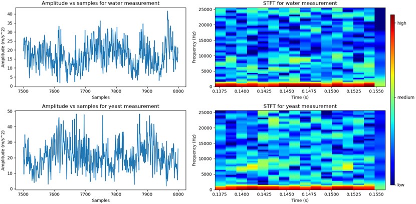
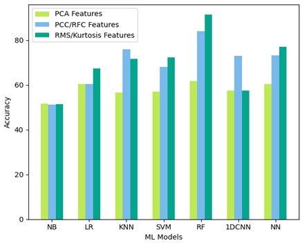
To evaluate the performance of the trained model, we used 2,316 data points (20 % of the overall data points) as test data among which 1,126 data points were from yeast measurements. Fig. 3 depicts the accuracy of the ML models for three feature engineering strategies. An accuracy of at least 75 % is considered as sufficient. With an accuracy of 91.27 %, RF outperforms the other categorization models using the feature set with RMS and kurtosis. The second highest accuracy is RF using the seven features from PCC/RFC with a value of 84.01 %. NN reached 76.95 % accuracy using the RMS/kurtosis feature set and KNN reached 75.86 % with the PCC/RFC feature set. The models using the PCA feature set were not able to reach the accuracy threshold.
Other performance indicators, such as precision, recall, f1-score, and specificity, were also examined to determine whether the models could perform the classification correctly. Taking yeast as positive, the metrics can be described as follows:
Fig. 3Accuracy of applied classification models
The metrics for each of the models are shown in Table 2 for the PCA feature set, in Table 3 for the PCC/RFC feature set and in Table 4 for the RMS/kurtosis feature set. The analysis of the metrics reveals that the RMS/kurtosis feature set provides the best results, directly followed by the PCC/RFC feature set. The PCA feature set was not able to classify the conditions good enough.
Table 2Performance metrics of ML models considering 4 PCA components as feature
Evaluated metrics | Classification models | ||||||
NB | LR | KNN | SVM | RF | 1DCNN | NN | |
Precision | 0.92 | 0.89 | 0.51 | 0.83 | 0.64 | 0.72 | 0.62 |
Recall | 0.51 | 0.52 | 0.57 | 0.55 | 0.62 | 0.55 | 0.64 |
Accuracy (%) | 51.63 | 60.43 | 56.58 | 57.09 | 61.61 | 57.34 | 60.28 |
F1-score | 0.65 | 0.65 | 0.53 | 0.67 | 0.63 | 0.62 | 0.62 |
Specificity | 0.56 | 0.59 | 0.56 | 0.63 | 0.61 | 0.57 | 0.59 |
Table 3Performance metrics of ML models considering 7 features using correlation and relevance
Evaluated metrics | Classification models | ||||||
NB | LR | KNN | SVM | RF | 1DCNN | NN | |
Precision | 0.04 | 0.72 | 0.80 | 0.85 | 0.90 | 0.72 | 0.74 |
Recall | 0.51 | 0.58 | 0.79 | 0.64 | 0.80 | 0.70 | 0.73 |
Accuracy (%) | 51.03 | 60.43 | 75.86 | 67.92 | 84.01 | 72.89 | 73.25 |
F1-score | 0.07 | 0.64 | 0.79 | 0.73 | 0.84 | 0.73 | 0.79 |
Specificity | 0.19 | 0.63 | 0.78 | 0.77 | 0.88 | 0.71 | 0.73 |
It’s essential to note that these models needed to be tuned with suitable hyperparameters. The adjustment of the hyperparameters appeared to increase the performance by almost 5 % on average.
Table 4Performance metrics of ML models considering 10 features using RMS & kurtosis
Evaluated metrics | Classification models | ||||||
NB | LR | KNN | SVM | RF | 1DCNN | NN | |
Precision | 0.10 | 0.82 | 0.72 | 0.68 | 0.95 | 0.78 | 0.86 |
Recall | 0.61 | 0.63 | 0.71 | 0.75 | 0.88 | 0.56 | 0.73 |
Accuracy (%) | 51.35 | 67.35 | 71.53 | 72.3 | 91.27 | 57.34 | 76.95 |
F1-score | 0.21 | 0.72 | 0.72 | 0.71 | 0.92 | 0.65 | 0.79 |
Specificity | 0.50 | 0.74 | 0.71 | 0.70 | 0.94 | 0.82 | 0.62 |
5. Conclusions
By analyzing vibration data, we found out that it is possible to determine, if only water or in addition also yeast is fed to a disk stack separator. We used seven ML models in combination with three different feature engineering strategies, leading to a total amount of 21 binary classification models. With four of our models, we reached an accuracy of more than 75 %. It turned out, that the manually selected features (RMS and kurtosis) provided the best results with an accuracy of 91.27 % in combination with a random forest classifier. It shows that considering domain specific knowledge about suitable feature selection techniques can provide better results than using PCA or correlation-based feature selection algorithms.
References
-
D. Goyal Vanraj, A. Saini, S. S. Dhami, and B. S. Pabla, “Intelligent predictive maintenance of dynamic systems using condition monitoring and signal processing techniques – A review,” in International Conference on Advances in Computing, Communication, and Automation (ICACCA), 2016.
-
M. Z. Ali, M. N. S. K. Shabbir, X. Liang, Y. Zhang, and T. Hu, “Machine learning-based fault diagnosis for single – and multi-faults in induction motors using measured stator currents and vibration signals,” IEEE Transactions on Industry Applications, Vol. 55, No. 3, pp. 2378–2391, May 2019, https://doi.org/10.1109/tia.2019.2895797
-
D. Siano and M. A. Panza, “Diagnostic method by using vibration analysis for pump fault detection,” Energy Procedia, Vol. 148, pp. 10–17, Aug. 2018, https://doi.org/10.1016/j.egypro.2018.08.013
-
H. Liu, L. Li, and J. Ma, “Rolling bearing fault diagnosis based on STFT-deep learning and sound signals,” Shock and Vibration, Vol. 2016, pp. 1–12, 2016, https://doi.org/10.1155/2016/6127479
-
A. Arcos Jiménez, C. Q. Gómez Muñoz, and F. P. García Márquez, “Dirt and mud detection and diagnosis on a wind turbine blade employing guided waves and supervised learning classifiers,” Reliability Engineering and System Safety, Vol. 184, pp. 2–12, Apr. 2019, https://doi.org/10.1016/j.ress.2018.02.013
-
R. Dumitrescu and M. Fleuter, Intelligenter Separator: Optimale Veredelung von Lebensmitteln. Berlin, Heidelberg: Springer Vieweg, 2019.
-
A. Kanawaday and A. Sane, “Machine learning for predictive maintenance of industrial machines using IoT sensor data,” in 8th IEEE International Conference on Software Engineering and Service Science (ICSESS), 2017.
-
A. Binding, N. Dykeman, and S. Pang, “Machine learning predictive maintenance on data in the wild,” in IEEE 5th World Forum on Internet of Things (WF-IoT), 2019.
-
E. Wallhäußer, W. B. Hussein, M. A. Hussein, J. Hinrichs, and T. Becker, “Detection of dairy fouling: Combining ultrasonic measurements and classification methods,” Engineering in Life Sciences, Vol. 13, No. 3, pp. 292–301, May 2013, https://doi.org/10.1002/elsc.201200081
-
L. Eren, “Bearing fault detection by one-dimensional convolutional neural networks,” Mathematical Problems in Engineering, Vol. 2017, pp. 1–9, 2017, https://doi.org/10.1155/2017/8617315
-
J. Ben Ali, B. Chebel-Morello, L. Saidi, S. Malinowski, and F. Fnaiech, “Accurate bearing remaining useful life prediction based on Weibull distribution and artificial neural network,” Mechanical Systems and Signal Processing, Vol. 56-57, pp. 150–172, May 2015, https://doi.org/10.1016/j.ymssp.2014.10.014
-
F. Pedregosafabian et al., “Scikit-learn: machine learning in Python,” The Journal of Machine Learning Research, Nov. 2011.
Cited by
About this article

The work in this paper was supported by the German Federal Ministry for Economic Affairs and Climate Action under grant 03EN4004B.
The datasets generated during and/or analyzed during the current study are available from the corresponding author on reasonable request.
The authors declare that they have no conflict of interest.
