Abstract
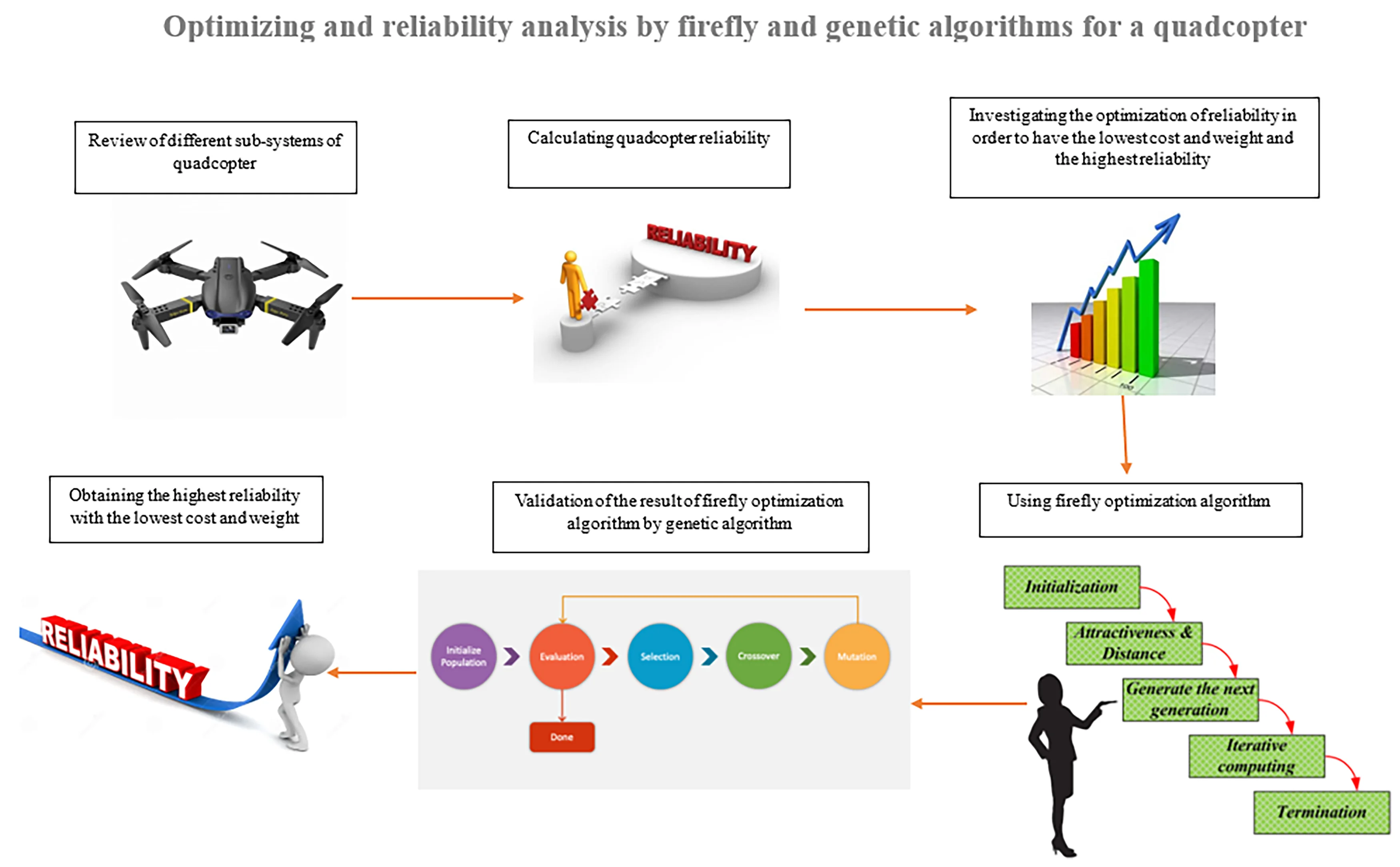
Our study aims to obtain the highest level of reliability for a quadcopter, taking financial and mass limitations into account, to achieve the highest level of reliability with the lowest mass and cost. For this purpose, we first calculated the reliability and the relationships that govern it, and based on these relationships, we determined the reliability of the quadcopter subsystems. In order to achieve the highest level of reliability, we utilized optimization algorithms. It is possible to increase the reliability of a system through several methods, such as enhancing the quality of parts and components, using surplus components, improving the quality of parts and components by always using surplus components, and redesigning the system. This study examines the possibility of increasing quadcopter reliability by using additional parts and optimizing it using the firefly algorithm. Lastly, in order to validate the results obtained from the firefly algorithm, we implemented the problem once again using the genetic algorithm and compared the results obtained from both algorithms. After 20 times of running the algorithms, the optimal reliability values were 0.99925 for the firefly algorithm and 0.99999 for the genetic algorithm.
Highlights
- reliability is the probability of satisfactory performance of the system under specific working conditions for a particular time. It is reliability.
- Optimization is the art of finding the best solution among existing situations. The innate desire of every human being to reach perfection shows the theory of optimization.
- Firefly Algorithm is an innovative algorithm inspired by the light emitting behavior of fireflies.
1. Introduction
Engineering and technical management are essential components of every modern society. They are responsible for planning, designing, constructing, and maintaining everything from the most specific product to the most complex systems. System failures result in disruptions on multiple levels and can even threaten society and the environment. Therefore, consumers expect reliable and safe products and systems [1].
There are different definitions of reliability, which can be defined as the probability that the device will not fail until a sure time , the average operating time of a device between two consecutive failures, the continuity of operation without failure, the probability of a device or system remaining in a functional condition without occurrence. Nevertheless, in the end, the complete definition of reliability is the probability of satisfactory performance of the system under specific working conditions for a particular time. It is reliability. The mathematical definition of probability states that it is a numerical index whose value can be from zero to one. When the probability is equal to zero, it means that there is no possibility of occurrence, and when it is one, it means that the occurrence is particular.
Nevertheless, in the other three sections, including satisfactory performance, time, and certain working conditions, which are all engineering parameters, probability theory does not help in any way, and only engineers and experts can provide information related to satisfactory performance and time may be continuous, or discontinuity may be considered. Finally, the work conditions may be wholly uniform or strongly changing. Therefore, probability theory is only a tool to convert the information of a system into possible performance prediction [1-3].
On the other hand, today, we are witnessing the emergence of a new and different generation of birds in the aviation industry, which has caused tremendous changes in this field. Among this new equipment, quadcopters, which due to their particular characteristics, such as high stability, controllability, small dimensions, etc., have caused it to play many roles in various industries. Several high-tech elements are contained in quadcopters, as well as specific flight standards, which make them highly functional. According to their estimates, any failure or defect will incur a great deal of expense, no matter how small. Therefore, reliability estimation is of particular importance for these systems [1, 4].
Also, it is impossible to improve reliability in any way because our financial resources are limited, and we also cannot increase the mass of the system beyond the permissible limit because we will have problems in flight. Therefore, we need to optimize the reliability. Consequently, we can achieve the best possible reliability by spending the least financial and criminal resources [5].
In this research, to increase the quality and performance of the quadcopter and reduce financial costs, we want to investigate the reliability of the electronic board and printed circuit. Then we optimized the reliability of its electronic board using the firefly algorithm and validated the results obtained using the genetic algorithm. Also, this work is about calculating the reliability of electronic components as well as optimizing reliability with the firefly algorithm for innovative quadcopters.
1.1. Background research
Reliability is an old concept and a new discipline, which has been the focus of engineers in many industries today for the development and improvement of quality. Reliability assessment methods in terms of the history of their origin, first in connection with the aerospace industry and during World War I. The second was done for German rockets in a preliminary way, but it was quickly noticed in other industries, such as the nuclear industry, which was under intense pressure to ensure the safety of nuclear reactors to provide electrical energy.
Several years after the United States launched its first satellite, statistical analyses of reliability and orbital failures were developed. In 1973, Krishna Behari Misra introduced the concepts of reliability and cost. The concept of reliability suggests many methods for optimal design of a system under certain conditions. In most of the articles, the main issue is assigning reliability to the components of the system and optimizing it based on bounded information. This process is a partial optimization for reliability. In the design phase, a designer has many options for system design. These options include increasing the reliability level of components and using extra components. A correct optimal system design examines all these options. Throughout the feasibility article Satisfying the optimal design is followed by cost constraints and the use of supporting components [6].
Kamal Kumar Govil investigated issues of partial reliability, discrete points of cost, and reliability. Also, placing these discrete data in a standard chart is necessary and vital. In this article, by using the least squares method, the crucial relationships of reliability and cost are expanded for use in problems with discrete data [7].
To increase reliability of series-parallel systems, plug-in components are used in the optimization plan, referred to as the redundancy allocation problem. In order to increase reliability concepts and components while taking into account limitations such as volume and weight, this problem aims to increase reliability concepts and components. The series-parallel structure is one of the types of system structures that is designed by allocating redundant components in parallel to the components of a system with a series structure [8].
Ku et al. stated in an article in 2000 that, in general, reliability can be defined as the long-term quality or the probability of a system's optimal performance under certain operational conditions in a certain period of time [9].
Zigo et al. designed a multi-objective optimization model for the reliability optimization problem through the allocation of additional components with transformation intensification. They solve the problem using a genetic algorithm [10].
In 2012, Joseph Homer Saleh et al. analyzed the reliability and failure of satellite electronic subsystems and their improvement through redundancy [11].
Additionally, in 2022, Tripti Dahiya et al. tried to improve the reliability of a system by combining two optimization algorithms, PSO and GA, in an article called Reliability optimization using hybrid genetic and particle swarm optimization algorithm [12].
Kazem Imani et. al. published a paper in 2022 in which they tried to calculate the reliability of a quadcopter power distribution [13].
1.2. Reliability indicators
The classic index of reliability, as mentioned, is the probability of failure, but many other indicators are also used for this purpose today, which depends on the type of system and their operational requirements, some of which are mentioned below [1, 14]: 1 – The number of expected failures in a certain time range. 2 – The average time between failures. 3 – Expected loss in investment due to failure. 4 – Expected reduction in system output due to various types of malfunctions. Each of these indicators can be evaluated using the relevant theory of reliability, and their selection will depend on the type of problem [15].
1.3. Types of system configuration
A system includes a network of components that are connected to each other in series, parallel, series-parallel combination and complex.
1.3.1. Series configuration
In series mode, all components of the system are considered critical, in other words, the failure of one component will cause the entire system to stop and fail.
If system reliability and the reliability of the n component with are shown and n components of the system are considered independent of each other, then the following relationship is established in the series mode:
As a result, the reliability of the system will not be greater than the lowest reliability of the components, so according to the above relationship, in order to achieve high reliability for a system with series components, the high reliability of each component is very important. If the failure rate of each component is constant and equal to, the reliability of the system is calculated as Eq. (1) [1, 16]:
1.3.2. Parallel configuration
The combination of two or more components that are parallel to each other or, in other words, redundant members of each other, is called a parallel system. In this configuration, the system stops or crashes when all the components fail, and as long as at least one component performs optimally, the system will continue to work. System reliability For parallel and independent components, it is obtained from the Eq. (2):
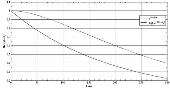
The reliability graph of the two supporting members is convex at the beginning of the time range. In comparison, the same graph for the single component is concave in the entire time range compared to the origin of the calculations. This difference is well shown in Fig. 1. In this figure, the failure rate for both modes, it is 0.005 per unit of time [1, 17, 18].
Fig. 1Reliability changes in parallel and single system
1.4. Combined series-parallel configuration
This system includes both series and parallel relationships between components. An example of a combined system is shown in Fig. 2.
Fig. 2Combined series-parallel configuration
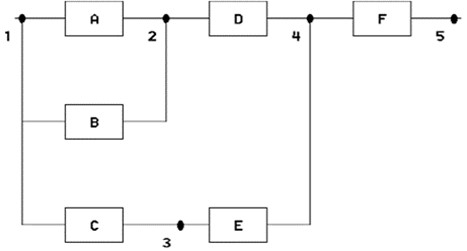
To calculate the reliability of the system, the network is broken into several sets, then the reliability of each set is calculated, and then the reliability of the system is obtained from the relationship of the reliability values of each set. In Fig. 7, the reliability is calculated as follows [3, 18]:
1.4.1. Optimization
Optimization is the art of finding the best solution among existing situations. The innate desire of every human being to reach perfection shows the theory of optimization. Man wants to visualize and describe the best and achieve it, but since he knows that he cannot identify and define well all the conditions governing the best, in most cases, instead of the best or absolute optimal answer, he finds a satisfactory answer. Optimization is an important tool in the decision-making and analysis of physical systems. Mathematically, an optimization problem is a problem of finding the best solution among a set of candidates or possible solutions. In this and similar cases, since more than one objective function must be considered, it is necessary to consider the application of multi-objective optimization methods. The most important feature of such methods is that by using multi-objective optimization models, more than one candidate solution is available to system designers and engineers; Each of these answers will display the balance between different objective functions [16].
1.4.2. Multi-objective optimization
Multi-objective optimization methods are used in many branches of science and engineering when a balance needs to be established between two or more conflicting objectives to reach optimal decisions in the system. Undoubtedly, in many engineering applications, designers of engineering processes and systems make decisions based on conflicting goals. For example, in the process of designing a car, in addition to the fact that engineers aim to design a car with maximum performance, at the same time, they seek to design a car with the lowest number of emissions and fuel consumption.
2. Methodology
2.1. Reliability prediction
Special relationships are used to predict the failure rate of components or systems correctly. These relationships have been developed with statistical models and based on environmental parameters affecting the performance of components. Two crucial standards, NSWC-98/LEI for mechanical parts and MIL HNBK- 217 for electronic components and the IEC-62380 document, have fully expanded these relationships. In this project, the MIL HNBK-21 standard and the IEC-62380 document have advanced the reliability plan.
2.2. Calculating quadcopter reliability
In calculating the reliability, estimating the failure rate of parts is very important. Calculating this number is very expensive for companies producing parts due to the complexity and variety of lifetime tests. As a result, in most cases, the failure rate of parts is not recorded in their information table. This makes it difficult to calculate the reliability of the quadcopter. To overcome this problem, alternative methods are used to calculate the failure rate of these parts. One of these methods, which is used for electronic parts, is reliability prediction based on models. Statistics have expanded. Another method is the method of assigning reliability to each of the components, which is achieved according to the influencing parameters of a system, including complexity, technology, environmental conditions, and performance time. Here we consider the operational life of the quadcopter as 3 years [19, 20].
2.3. Optimization methods
Optimization methods and algorithms are divided into two categories: exact and approximate algorithms. Approximate algorithms are divided into two categories: heuristic and meta-heuristic algorithms. In the exact method, we have a series of algorithms that can give a completely accurate and definitive answer by searching and viewing all the data. These algorithms have low speed and naturally, they are not very useful for problems with large data and dimensions. On the other hand, in the approximate method, there are another series of algorithms that can search specific parts of the data by using the initiative, and by doing so, they increase the speed of generating the answer. Although, this is heuristic algorithms do not guarantee that the obtained answer is the best possible answer. That is, if you search further, you will probably find a better answer. The biggest problem of the heuristic method is that it needs to know the problem. In other words, an innovative algorithm will be responsible for a specific problem. Another problem of heuristic algorithms is their getting stuck in local optimal points, and premature convergence to these points, and here another series of algorithms have been created that can search for optimal points without having the problems of heuristic methods. Indeed, meta-heuristic algorithms are able to solve the problem with reasonable speed and accuracy by providing a general solution without knowing the problem. These methods are in the term independent of the problem [5].
2.3.1. Firefly algorithm (FA)
Firefly Algorithm is an innovative algorithm inspired by the light emitting behavior of fireflies. The algorithm is an evolutionary model based on collective intelligence which was derived from nature. The main application of this algorithm is solving optimization problems. In order to increase the search power, accuracy of the algorithm, and improve the resulting result, an improved firefly algorithm is used by changing how the firefly moves and increasing the convergence in the global optimum. According to the type of optimization, the optimal point can be the particle that has the highest or the lowest value, and the value of this particle is updated every time it is repeated. In the proposed algorithm, when two values or two positions are compared, the new location will be obtained according to the location of the current two values, and a new result will be attained from the difference of the best and worst value in the global optimum. This move will escape from the worst situation in the algorithm and will lead the algorithm to the global optimal solution. The firefly algorithm was introduced in late 2007 by Xin-She Yang, whose main idea was inspired by the optical communication between fireflies. This algorithm can be seen as a manifestation of collective intelligence, in which a higher level of intelligence is created from the cooperation of simple and low-intelligence members, which definitely cannot be achieved by any of the components. The FA algorithm is a meta-heuristic algorithm inspired by the behavior of fireflies. This algorithm has been formulated with the following hypothesis: 1 – All fireflies are sexual so one firefly attracts all other fireflies. 2 – The attractiveness is proportional to the brightness of the worm, and usually fireflies with less light are attracted to brighter fireflies. 3 – If there is a firefly brighter than the given firefly, it will move randomly. 4 – Lighting must be related to the objective function.
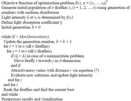
The firefly algorithm by modeling the behavior of a set of fireflies and assigning a value related to the fitness of the location of each firefly as a model for the amount of firefly pigments and updating the locations of the fireflies in successive iterations of the algorithm to search for the optimal solution The problem is solved. In fact, the two main steps of the algorithm in each iteration are the pigment updating phase and the movement phase. Fireflies move towards other fireflies with more pigment in their neighborhood. In this way, during successive iterations, the collection tends towards a better answer. According to the algorithm and flowchart, we can implement this optimization for the problem of reliability [1, 21-24].
The procedure for implementing the FA algorithm can be as the code in Fig. 3.
2.4. Problem statement
The firefly algorithm is a new population-based multivariate approach developed by Xin-She Yang and inspired by the behavior of the blinking properties of fireflies. The flickering light can be formulated in such a way that it is accompanied by an optimized objective function, which enables the formulation of the firefly algorithm. To implement this algorithm for a board, we consider a quadcopter that includes six main components, each component is marked with a number as follows. For this purpose, we consider four main components and each index represents one of the components. These are the four components in order: 1 – flash memory, 2 – driver, 3 –transmitter and receiver, 4 – processor, 5 – flow sensor, 6 – temperature sensor.
In this problem, the weight function, the cost function, and the objective function are known, and the relationships and correlations between them are known. We should get the most optimal mode for reliability by running the program and determining the different modes of redundancy in order to have the most optimal mode according to the weight and cost limitations. In this case, the maximum weight is 5000 grams and the maximum cost is 3500 dollars. Next, in order to validate the firefly program, we implement this program in Toolbox Optimization of MATLAB software by genetic algorithm and compare the results.
Fig. 3Algorithm of the FA
The reliability-redundancy assignment problem to maximize the system reliability by considering the constraints can be formulated as follows:
In this research, we are looking for multi-objective optimization. We want to have maximum reliability with minimum cost and weight for our quadcopter. The following function should be maximized Also considering , , , , where in. Subsystem reliability, g are a set of constraint functions (weight and cost functions), ). Reliability vector of subsystem components and are the vector of redundancies assigned to the subsystem. and . The reliability and number of components of each subsystem is in the -th component of the subsystem. For example, The total number of flash memory (main + spare) and . The amount of reliability of flash memory. The objective function for all reliability of the subsystem, l is the resource limitation of the subsystem and m is the number of components of each member in the subsystem. This problem is a series of mixed-integer nonlinear problems. The problem can be started as follows:
The function should be maximized. Considering the weight function , and cost function, , where in and and and and the limit of the cost (budget). Here, is the desired part number in the subsystem. For example, represents the total number of flash memories (main + surplus) and indicates the reliability of flash memories with the number considered is the component cost function where is the operating time of each subsystem component in which it does not fail. is also an upper limit of the weight of the subsystem. It’s derived from the fault tree analysis of the subsystems’ structure diagrams. Since the attractiveness of a firefly is proportional to the intensity of light seen by neighboring fireflies, we can now define the attractiveness of a firefly in terms of the Cartesian distance between firefly and firefly . In this case, the distance of the -th firefly to the more attractive (brighter) -th firefly that is attracted to it, is Eq. (3):
The second part is related to the attractiveness of fireflies, where is the absorption coefficient of fireflies, absorption coefficient in . In the third part, we are looking to create random numbers using the coefficient. The generated random number is between 0 and 1.
2.5. Structure of the manuscript
In the continuation of the Results section, it is divided into two sections: component reliability calculation and optimization section. In the reliability section, we examine the components of the quadcopter and calculate the reliability of the various parts of the quadcopter using the failure rate and existing relationships and tables.
Next, in the optimization section, we will first explain the parameters and the algorithm, and then we will express the results of the firefly algorithm. Finally, we use the genetic algorithm to validate the result of the firefly algorithm.
In the Conclusion section, we have compared the results of firefly and genetics algorithms and we have displayed the results of the comparison under the title of Table 9.
3. Results
3.1. Reliability
3.1.1. Estimating the reliability of command board
The command and data management board includes several main and vital components that are placed on the printed circuit fiber. Next, the reliability of the important components and the printed circuit fiber is calculated. After calculating the reliability of various components, the reliability of the data command management board is calculated using the following relationship [4]:
3.1.1.1. Processor
In order to design and build the command and data management board, a processor with good processing power and at the same time low power consumption, which has a hardware decimal computing unit, should be used. This processor is designed to be used in applications with high power consumption. This processor uses the ARM-Cortex R4F architecture and is a product of Texas Instruments. The FIT value of this part is 41.2. In order to design and build the command and data management board, a processor with good processing power and at the same time low power consumption, which has a hardware decimal computing unit, should be used. This processor is designed to be used in applications with high power consumption. This processor uses the ARM-Cortex R4F architecture and is a product of Texas Instruments. The FIT value of this part is 2.41. The component reliability is calculated as follows:
3.1.1.2. AT45 flash memory
This part is made in Atmel technology company. The information of the various components of the quadcopter is stored in this part. The FIT of this part is equal to 1.3. The reliability of this part is calculated as follows:
3.1.1.3. Sender and receiver
This part is a product of Texas Instruments company with FIT 4.65. The reliability of this part can be calculated as follows:
3.1.1.4. Motor driver
This part is a product of Analog Device company with FIT 1.44. The reliability of this part is calculated as follows:
The reliability of the command board and data management components along with the number of parts are listed in the Table 1.
Table 1Reliability of electrical components
Part type | FIT | Reliability | Number of parts |
Flash memory | 1.3 | 0.9999985762 | 1 |
Driver | 1.44 | 0.9999998423 | 2 |
Sender and receiver | 4.65 | 0.9999994908 | 1 |
Processor | 2.41 | 0.9999762494 | 1 |
Flow sensor | 2.7 | 0.9999970437 | 1 |
Temperature sensor | 3 | 0.9999967155 | 1 |
ECS | 1.5 | 0.9999983516 | 1 |
Now, if we consider redundancy for some important components, their reliability changes as follows (Number of components = number of main components + redundancy).
Table 2Redundancy for some important components
Flash memory | |||
Number of components (n) | 2 | 3 | 4 |
Reliability (r) | 0.9999991624 | 0.999994774 | 0.9999997485 |
Driver | |||
Number of components (n) | 2 | 3 | 4 |
Reliability (r) | 0.9999986554 | 0.9999989546 | 0.9999991542 |
Sender and Receiver | |||
Number of components(n) | 2 | 3 | 4 |
Reliability(r) | 0.9999996542 | 0.9999997562 | 0.99999998545 |
Processor | |||
Number of components (n) | 2 | 3 | 4 |
Reliability (r) | 0.999980215 | 0.999982654 | 0.999985423 |
Flow sensor | |||
Number of components (n) | 2 | 3 | 4 |
Reliability (r) | 0.9999975364 | 0.9999977332 | 0.999997866 |
Temperature sensor | |||
Number of components (n) | 2 | 3 | 4 |
Reliability (r) | 0.9999971344 | 0.9999974352 | 0.9999978999 |
ECS | |||
Number of components(n) | 2 | 3 | 4 |
Reliability(r) | 0.999998644 | 0.9999990444 | 0.999999235 |
Finally, the reliability of the command board is equal to 0.999999456.
3.1.2. Reliability estimation of printed circuit fiber and connections
3.1.2.1. Estimating the reliability of connections
The reliability between the board and the components are sensitive to heat and the type of connections. The sensitivity can be expressed in the form of Eq. (4) [19], [25], [26]:
Table 3Connections on board [25-27]
Effective coefficient | 8760 Cycles/Year | ||
8760 Cycles/Year | |||
: Number of cycles including turning the board off and on in a year with temperature range of | |||
: Outdoor environment temperature in the th phase of operation | : Indoor environment temperature, near the components in the th phase of operation | ||
For solder joints in each 1 billion hours equal 0.5 | |||
Due to the small space of the board and box, the temperature of the environment near the components is the same as the temperature around the board. As a result, the failure rate and reliability of connections are:
The reliability of a printed circuit fiber depends on the area of the fiber openings, the number of circuit layers, the width of the signal path on the board and the number of connections:
Coefficients and impact factors can be calculated using the Table 4.
Table 4Effective coefficients and factors in calculating the reliability of printed circuit fiber [27]
Effective coefficient | Number of Layers ≤ 2 | 1 | |||
Number of Layers > 2 | 0.7 × | ||||
: Number of Signal Paths : Number of holes in the board : Board Area (120 cm2) | |||||
0.56 | 0.35 | 0.23 | 0.15 | 0.1 | Width of the maximum flow path |
1 | 2 | 3 | 4 | 5 | |
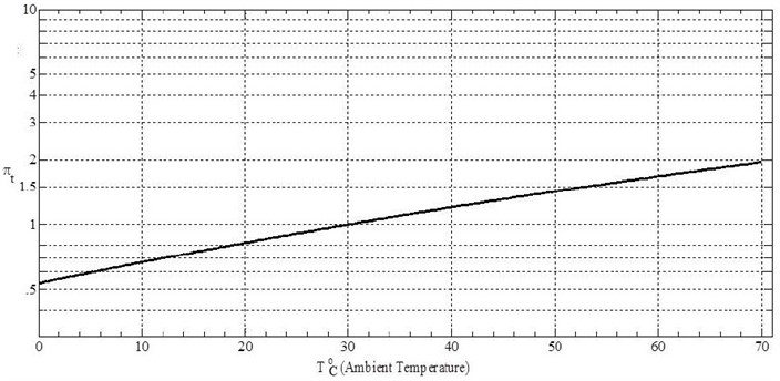
For the proper analysis of the temperature coefficient, the maximum temperature of the device must be taken into account, and for this purpose, the diagram in Fig. 4 is used:
The fiber printed circuit board for the control board has 19 apertures, including embedded apertures for screws, connecting parts and connectors. Also, there are 53 signal paths in all layers of the board to connect different parts. According to Eq. (5):
Finally, the reliability of printed circuit fiber is equal to:
Fig. 4Temperature factor changes in the range of 0-70 degrees Celsius
3.1.3. Battery
The SB (Storage battery) in the quadcopter is the only generator of electrical energy. Most of the batteries are of the lithium polymer (LiPo) type. The reason for using these BC (Battery cells) is because of their high energy density and high discharge rate. The reliability relationship of the SB part is defined as Eq. (6) [27]:
where is the number of batteries, which is equal to 4, and is the excess number of batteries which is equal to one:
From an analysis of possible sudden failures of such sections, the following failures generated lead to a complete failure of each section [27].
Now the reliability equation of each battery is as follows:
where is Reliability of batteries not being damaged, and is Reliability of not shorting circuit the batteries, and is Reliability of not breaking down CEU.so:
finally, the price of each used lithium-ion battery is, so: 100 $.
3.2. Optimization
3.2.1. Firefly algorithm
By running the firefly algorithm in the MATLAB environment 20 times, with a system by CPU Intel CORE i7 5500U 2 Core 3.40 Ghz and RAM 8 GB 1600 MHz in windows8, the results of Table 5 and Table 6 were obtained, which show the different optimized parameters, where is from 1 to six in the following order: 1 – flash memory, 2 – driver, 3 – transmitter and receiver, 4 – processor, 5 – current sensor, 6 – temperature sensor.
Table 5Conclusion 1 reliability optimization by FA algorithm
Parameters | Execution number | |||||||||
1 | 2 | 3 | 4 | 5 | 6 | 7 | 8 | 9 | 10 | |
3 | 2 | 3 | 2 | 4 | 2 | 2 | 3 | 4 | 4 | |
3 | 4 | 3 | 3 | 4 | 2 | 2 | 3 | 3 | 4 | |
3 | 4 | 4 | 2 | 2 | 3 | 2 | 4 | 4 | 2 | |
2 | 4 | 3 | 4 | 2 | 2 | 2 | 3 | 4 | 4 | |
2 | 2 | 3 | 2 | 3 | 3 | 3 | 2 | 2 | 3 | |
2 | 3 | 3 | 3 | 3 | 3 | 4 | 2 | 2 | 2 | |
Cost | 3464.43 | 3402.82 | 3461.87 | 3466.38 | 3415.55 | 3439.11 | 3468.86 | 3406.48 | 3462.99 | 3461.97 |
Weight | 4765.53 | 4595.40 | 4706.44 | 4769.21 | 4581.47 | 4792.78 | 4828.23 | 4733.45 | 4568.77 | 4617.93 |
Best firefly | 0.98783 | 0.99615 | 0.99279 | 0.9901 | 0.99925 | 0.94995 | 0.9813 | 0.9930 | 0.9962 | 0.99044 |
Table 6Conclusion 2 reliability optimization by FA algorithm
Parameters | Execution number | |||||||||
11 | 12 | 13 | 14 | 15 | 16 | 17 | 18 | 19 | 20 | |
3 | 4 | 4 | 4 | 3 | 3 | 4 | 3 | 4 | 3 | |
2 | 4 | 4 | 2 | 3 | 2 | 4 | 3 | 3 | 3 | |
3 | 4 | 4 | 4 | 2 | 4 | 3 | 4 | 2 | 4 | |
2 | 3 | 3 | 2 | 3 | 2 | 2 | 3 | 4 | 4 | |
2 | 2 | 3 | 2 | 2 | 3 | 3 | 4 | 2 | 3 | |
3 | 3 | 4 | 2 | 2 | 4 | 2 | 4 | 2 | 4 | |
Cost | 3456.88 | 3476.27 | 3484.54 | 3460.77 | 3485.68 | 3433.62 | 3422.03 | 3428.47 | 3249.15 | 3441.77 |
Weight | 4746.58 | 4554.85 | 4647.48 | 4821.39 | 4722.60 | 4623.11 | 4928.60 | 4463.79 | 4620.90 | 4627.7 |
Best firefly | 0.94675 | 0.99757 | 0.98883 | 0.99027 | 0.98244 | 0.99765 | 0.99143 | 0.97011 | 0.99757 | 0.99431 |
According to these results, it can be concluded that the best mode (Best Firefly) has been obtained in the fifth execution of the program, which gives us a reliability of 0.99925. 3 will be surplus. Also, we will have 4 drivers, 2 of which will be main and 2 surpluses. Also, 2 transmitters and receivers, 1 of which will be main and 1 surplus. 2 processors, one the main number and one surplus. 3 flow sensors, one main and 2 surpluses. Finally, 3 temperature sensors, one main and 2 surpluses. The total cost of the subsystem will be 3415.15 dollars and the total weight of the subsystem will be 4620.9 grams [21], [24].
3.2.2. Genetic algorithm optimization results in optimization toolbox MATLAB
In this case, like FA in the environment of MATLAB version 2020, with a system by CPU Intel CORE i7 5500U 2 Core 3.40 GHz and RAM 8 GB 1600 MHz in windows8, we run the program 20 times and report the results. In the optimization of our problem, for algorithms with a large amount of data, the genetic algorithm is efficient., the following 12 parameters are considered as variables [26]: , , , , , , , , , , , .
The upper and lower ranges of each of these variables are also shown in Table 7.
Table 7Upper and lower ranges of variables in genetic algorithm
Parameters | ||||||||||||
Lower Bound | 1 | 1 | 1 | 1 | 1 | 1 | 0.5 | 0.5 | 0.5 | 0.5 | 0.5 | 0.5 |
Upper Bound | 3 | 3 | 4 | 3 | 4 | 3 | 0.999 | 0.999 | 0.899 | 0.999 | 0.999 | 0.999 |
The program code is written in MATLAB language and includes a main body that manages the inputs and outputs of the program. In this program, there is a counter that specifies how many calls to calculate the objective function are made by the code and how many are made by the history of the results. Also, if needed, the input data is read from the input files to start the optimization process. Also, the number of generations and the number of members of each generation are selected as the main inputs of the optimization process by the user, and the application specifies the minimum number of primary data to be present in the first population of primary data [28-31].
MaxGenerations_Data =1700; PopulationSize_Data = 1080’.
Table 8 and Table 9 show the results of the genetic algorithm.
Table 8Results 1 optimizing reliability by GOA algorithm
Parameters | Execution number | |||||||||
1 | 2 | 3 | 4 | 5 | 6 | 7 | 8 | 9 | 10 | |
4 | 4 | 3 | 3 | 3 | 4 | 3 | 2 | 2 | 4 | |
3 | 4 | 4 | 4 | 2 | 3 | 4 | 4 | 4 | 2 | |
4 | 4 | 4 | 4 | 4 | 2 | 4 | 3 | 4 | 3 | |
3 | 2 | 2 | 3 | 2 | 4 | 3 | 4 | 2 | 4 | |
4 | 4 | 4 | 4 | 4 | 4 | 2 | 4 | 4 | 4 | |
3 | 3 | 3 | 3 | 3 | 2 | 3 | 4 | 3 | 2 | |
Cost | 3464.18 | 3461.56 | 3480.88 | 3464.44 | 3464.44 | 3468.09 | 3461.18 | 3466.95 | 3468.43 | 3477.29 |
Weight | 4696.84 | 4710.64 | 4742.93 | 4762.25 | 4787.74 | 4831.74 | 4890.53 | 4716.62 | 4663.99 | 4875.72 |
Best Firefly | 0.96998 | 0.99201 | 0.98691 | 0.98745 | 0.98756 | 0.99924 | 0.99999 | 0.98103 | 0.98748 | 0.96355 |
Table 9Results 2 optimizing reliability by GOA algorithm
Parameters | Execution number | |||||||||
11 | 12 | 13 | 14 | 15 | 16 | 17 | 18 | 19 | 20 | |
4 | 4 | 4 | 3 | 2 | 4 | 2 | 4 | 4 | 2 | |
3 | 3 | 2 | 3 | 3 | 2 | 4 | 4 | 3 | 2 | |
4 | 2 | 4 | 4 | 4 | 4 | 3 | 3 | 4 | 4 | |
2 | 3 | 3 | 2 | 3 | 2 | 2 | 4 | 4 | 4 | |
3 | 2 | 2 | 4 | 2 | 3 | 2 | 3 | 3 | 2 | |
4 | 6 | 3 | 4 | 2 | 3 | 4 | 2 | 3 | 3 | |
Cost | 3454.38 | 3443.40 | 3348.69 | 3246.27 | 3446.52 | 3247.59 | 3246.79 | 3466.87 | 3347.82 | 3448.4 |
Weight | 4770.74 | 4657.41 | 4822.69 | 4921.67 | 4891.48 | 4672.57 | 4818.87 | 4570.42 | 4626.87 | 4265.3 |
In this case, the best choice was made in the seventh performance. In this case, we have three memory sticks, one of which is the main number and 2 of which will be redundant. We will also have four drivers, one of the main and 2 of which will be redundant. Also, there will be four transmitters and receivers, 1 of which is the main number and 3 of which will be redundant. It is surplus. 2 processors, one central number, and one redundant number. 2 flow sensors, one central number, and one redundant number. Finally, there will be three temperature sensors, one of which will be the main number, and two will be redundant. The total cost of the subsystem will be 3461.18 dollars, and the total weight of the subsystem will be 4890.53 grams.
3.2.3. 4. Discussion
Quadcopters are a new generation of drones that, due to their high technology, have unique features such as high controllability and extraordinary stability compared to other drones. This is why quadcopters are used in many industrial and commercial fields. take
Therefore, due to the high technology and extensive use, these devices must have sufficient reliability to minimize the risk of their failure and the costs caused by their failure. Nevertheless, in the discussion of reliability, we are always limited. We are facing
For example, in quadcopters, we face financial and weight restrictions because quadcopters, in order to have enough lift force, their weight should not exceed a certain amount, and we cannot add more parts or put parts of better quality but higher mass for to achieve more reliability.
Also, we always face financial constraints, and we must spend with limits to achieve more reliability. These things made us decide that in this research while obtaining the reliability of the quadcopter by optimizing it with the new meta-heuristic algorithm (Firefly algorithm) and validating the results with that classic meta-heuristic algorithm (genetic algorithm), we can obtain the maximum value Get reliability, the lowest cost and weight for it.
This is new research in quadcopter reliability with the view of optimizing reliability while minimizing weight and cost.
4. Conclusions
In this project, using applied methods, the failure rate and reliability of electric power subsystem components were investigated and compared with and without considering redundancies. Financial resources are limited for component designing, manufacturing, and assembling quadcopters. The cost of the subsystem components was calculated according to the prices listed on Amazon.com and electronic-shop.iu websites.
Nowadays, optimization in the engineering field has found a crucial role due to resource limitations. We also seek to get the highest efficiency by spending the least resources.
In recent years, with the emergence of meta-heuristic algorithms that are mostly modeled on nature, the optimization discussion has significantly progressed, the calculation time has been reduced, and the problem of local singular points in classical optimization has been fixed. We also have limitations regarding the reliability of the quadcopter, both in terms of financial cost and the weight of the components. To have the best possible state, we must optimize our resources.
In the optimization discussion, we used firefly algorithms (FA) and genetic algorithms (GOA) through the Toolbox Optimization section in MATLAB. Finally, the data obtained by the firefly algorithm can be validated by comparing the results of two firefly and genetic algorithms.
4.1. Limitation
In this research, we were faced with limitations in obtaining the failure rate of some parts, and with great effort, we succeeded in obtaining their values.
4.2. Recommendations
In future researches, other optimization algorithms can be investigated and the results compared with the results of the current research. Also, other UAVs can be investigated in terms of reliability and risk management.
Table 10Comparison of the results of FA and GOA algorithms
Parameters | FA | GOA | Data discrepancy |
4 | 3 | 1 | |
4 | 4 | 0 | |
2 | 4 | 2 | |
2 | 3 | 1 | |
3 | 2 | 1 | |
3 | 2 | 1 | |
Cost | 3451.55 | 3461.18 | 0.3 % |
Weight | 4581.47 | 4890.53 | 0.1 % |
Best | 0.99925 | 0.99999 | 0.07 % |
Therefore, by comparing the obtained answers, we can say that due to the closeness of the answers, we can ensure the correctness of the answers of the firefly algorithm.
References
-
R. Billinton and R. N. Allan, Reliability Evaluation of Engineering Systems. Boston, MA: Springer US, 1983, https://doi.org/10.1007/978-1-4615-7728-7
-
J.-F. Castet and J. H. Saleh, “Beyond reliability, multi-state failure analysis of satellite subsystems: A statistical approach,” Reliability Engineering and System Safety, Vol. 95, No. 4, pp. 311–322, Apr. 2010, https://doi.org/10.1016/j.ress.2009.11.001
-
A. Birolini, Reliability Engineering: Theory and Practice. Springer, 2004.
-
D. Papadimitriou et al., “Reliability based aerodynamic shape optimization of a quadcopter,” in 2018 AIAA Non-Deterministic Approaches Conference, Jan. 2018, https://doi.org/10.2514/6.2018-0664
-
A. M. Shaheen, S. R. Spea, S. M. Farrag, and M. A. Abido, “A review of meta-heuristic algorithms for reactive power planning problem,” Ain Shams Engineering Journal, Vol. 9, No. 2, pp. 215–231, Jun. 2018, https://doi.org/10.1016/j.asej.2015.12.003
-
K. B. Misra, “On optimal reliability design: a review,” IFAC Proceedings Volumes, Vol. 8, No. 1, pp. 27–36, Aug. 1975, https://doi.org/10.1016/s1474-6670(17)67533-5
-
Kamal Kumar Govil, “Fitting cost-reliability data in a standard curve,” Microelectronics Reliability, Vol. 25, No. 5, pp. 913–915, Jan. 1985, https://doi.org/10.1016/s0026-2714(85)80020-2
-
W.-C. Yeh and T.-J. Hsieh, “Solving reliability redundancy allocation problems using an artificial bee colony algorithm,” Computers and Operations Research, Vol. 38, No. 11, pp. 1465–1473, Nov. 2011, https://doi.org/10.1016/j.cor.2010.10.028
-
W. Kuo and V. R. Prasad, “An annotated overview of system-reliability optimization,” IEEE Transactions on Reliability, Vol. 49, No. 2, pp. 176–187, Jun. 2000, https://doi.org/10.1109/24.877336
-
Z. Zhang, Y. Xie, and Z. Yuan, “Multi-objective optimization design for output characteristics of LCC resonant converter,” in 2011 International Conference on Electrical Machines and Systems (ICEMS), Aug. 2011, https://doi.org/10.1109/icems.2011.6073415
-
S. Y. Kim, J.-F. Castet, and J. H. Saleh, “Spacecraft electrical power subsystem: Failure behavior, reliability, and multi-state failure analyses,” Reliability Engineering and System Safety, Vol. 98, No. 1, pp. 55–65, Feb. 2012, https://doi.org/10.1016/j.ress.2011.10.005
-
T. Dahiya and D. Garg, “Reliability optimization using hybrid genetic and particle swarm optimization algorithm,” Yugoslav Journal of Operations Research, Vol. 32, No. 4, pp. 439–452, 2022, https://doi.org/10.2298/yjor220316020d
-
K. Imani, A. Gholami, and M. Bagherian Dehaghi, “Reliability calculation with error tree analysis and breakdown effect analysis for a Quadcopter power distribution system,” Maintenance, Reliability and Condition Monitoring, Vol. 2, No. 2, pp. 45–57, Dec. 2022, https://doi.org/10.21595/marc.2022.23054
-
M. Farahmand, M. Ganji, and S. M. Sajadi, “Reliability evaluation and improvement of manufacturing helicopter in an aircraft manufacturing company – case study: skid types helicopter landing gear,” International Journal of Industrial and Systems Engineering, Vol. 31, No. 1, p. 95, 2019, https://doi.org/10.1504/ijise.2019.10017868
-
R. N. Allan and R. Billinton, “Concepts of power system reliability evaluation,” International Journal of Electrical Power and Energy Systems, Vol. 10, No. 3, pp. 139–141, Jul. 1988, https://doi.org/10.1016/0142-0615(88)90028-2
-
R. Tavakkoli-Moghaddam, J. Safari, and F. Sassani, “Reliability optimization of series-parallel systems with a choice of redundancy strategies using a genetic algorithm,” Reliability Engineering and System Safety, Vol. 93, No. 4, pp. 550–556, Apr. 2008, https://doi.org/10.1016/j.ress.2007.02.009
-
I. Häring, Technical Safety, Reliability and Resilience. Springer, 2021.
-
L. R. Lamberson, “Reliability Tutorial.,” Annual Quality Congress Transactions, Vol. 11, No. 5, pp. 88–89, 1985.
-
V. B. Larin, “Improving the reliability of the control system of a quadcopter,” International Applied Mechanics, Vol. 54, No. 4, pp. 454–462, Jul. 2018, https://doi.org/10.1007/s10778-018-0898-7
-
K. K. Aggarwal, K. B. Misra, and J. S. Gupta, “A fast algorithm for reliability evaluation,” IEEE Transactions on Reliability, Vol. R-24, No. 1, pp. 83–85, Apr. 1975, https://doi.org/10.1109/tr.1975.5215343
-
L. Dos Santos Coelho, D. L. de Andrade Bernert, and V. C. Mariani, “A chaotic firefly algorithm applied to reliability-redundancy optimization,” 2011 IEEE Congress on Evolutionary Computation (CEC), pp. 517–521, Jun. 2011, https://doi.org/10.1109/cec.2011.5949662
-
S. Kitaronka, “Optimization effects of Firefly algorithm in Smart Grids.pdf,” 2022.
-
K. Deb and H. Gupta, “Introducing robustness in multi-objective optimization,” Evolutionary Computation, Vol. 14, No. 4, pp. 463–494, Dec. 2006, https://doi.org/10.1162/evco.2006.14.4.463
-
D. K. Mishra, V. Shinde, and S. K. Bharadwaj, “A Convergence Study of Firefly Algorithm,” International Journal of Research in Science and Engineering, No. 23, pp. 17–25, May 2022, https://doi.org/10.55529/ijrise.23.17.25
-
“Handbook of Realibility Prediction for Mechanical Equepment,” Naval Undersea Warfare Center, 2010.
-
D. O. Defense, “Realibility Prediction of Electronic Equipment,” MIL-HDBK-217F, 1995.
-
M. B. A. Zahran and S. Sciences, “L.E.O. Satellite Power Subsystem Reliability Analysis,” Electronics Research Institute, 2014.
-
S. Katoch, S. S. Chauhan, and V. Kumar, “A review on genetic algorithm: past, present, and future,” Multimedia Tools and Applications, Vol. 80, No. 5, pp. 8091–8126, Feb. 2021, https://doi.org/10.1007/s11042-020-10139-6
-
R. Leardi, “Genetic algorithms,” Comprehensive Chemometrics, Vol. 1, pp. 631–653, 2009, https://doi.org/10.1016/b978-044452701-1.00039-9
-
A. Muñoz and F. Rubio, “Evaluating genetic algorithms through the approximability hierarchy,” Journal of Computational Science, Vol. 53, p. 101388, Jul. 2021, https://doi.org/10.1016/j.jocs.2021.101388
-
L. Morse, L. Cartabia, and V. Mallardo, “Reliability-based bottom-up manufacturing cost optimisation for composite aircraft structures,” Structural and Multidisciplinary Optimization, Vol. 65, No. 5, pp. 1–27, May 2022, https://doi.org/10.1007/s00158-022-03250-9
About this article

The authors have not disclosed any funding.
The datasets generated during and/or analyzed during the current study are available from the corresponding author on reasonable request.
Amirhossein Gholami assisted with conceptualization, data curation, investigation, methodology, writing original draft preparation, project, resources, validation, and visualization. Abolghasem Naghash contributed to supervision, administration, and methodology. Mahdi Bagherian Dehaghi contributed to writing review, and editing. Kazem Imanin contributed as a formal analyst.
The authors declare that they have no conflict of interest.
