Solitons in a cold electron beam plasma

1. Introduction

Dissipative electron-acoustic solitary waves (EASWs) in a cold electron beam plasma with superthermal trapped electrons are investigated in [1]. It is shown in [1] that EASWs can be described by the Shamel equation [2]:

where ${\mathrm{\Phi }}_1$ is the linearized electrostatic potential; ${\nu }_{c_0}$ is the cold electron-neutral collision frequency; $\tau$ and $\xi$ are time and spatial coordinates; $A$ and $B$ are system parameters representing properties of the normalized electron plasma. Eq. (1) shows stronger nonlinearity (due to the $\sqrt{{\mathrm{\Phi }}_1}$ term) as compared to the paradigmatic KdV equation.

Eq. (1) is reduced to:

In [1] by assuming the absence of the collision term $({\nu }_{c_0}=0)$. It is shown in [1] that using the boundary conditions ${\mathrm{\Phi }}_1\to 0$ and ${\mathrm{\Phi }}_1\xi \to 0$ at $\xi \to \pm \infty$, Eq. (2) produces EASWs through the following solution:

where $u_0$ is the propagation speed of the EASW; ${\mathrm{\Phi }}_m=(15u_0/8A{)}^2$ is the maximum amplitude and $\mathrm{\Delta }=\sqrt{16B/u_0}$ is the width of the EASW.

The main objective of this paper is to demonstrate that the solitary wave described by Eq. (3) does not satisfy Eq. (2) for all values of parameters $A$ and $B$, and for all initial (and boundary) conditions.

2. Preliminaries

3. Soliton solution to the Schamel equation

Consider the following differential equation:

Denoting $y={\sigma }^2{z}^2$ and differentiating Eq. (10) yields:

Eq. (11) can be rewritten in respect to $z$ in the following form:

Combining Eqs. (10) and (12) results in the following polynomial:

The values of $b_0,\dots ,b_3$ for which Eq. (11) is the extension of Eq. (10) are determined from Eq. (13):

As observed in [4], the solution to Eq. (10) satisfies Eq. (11) if and only if the initial conditions satisfy the following constraint:

Note that $b_1=0$ for the Schamel equation. Then special cases of Eq. (11) must be considered, because it follows from Eq. (15) that the parameters of Eq. (10) must satisfy the following relation:

4. Computational experiments

It can be seen from Eq. (22) that soliton solution Eq. (24) to Eq. (5) has a singularity if $b_3>0$. Further, only the soliton solution without singularity is considered.

Let us consider the following partial differential equation, as described in [1]:

Selecting the substitution $x=\xi +2\tau$ and denoting $y\left(x\right)=y\left(\xi +2\tau \right)={\mathrm{\Phi }}_1\left(\xi ,\tau \right)$ results in the following third-order ODE:

Integrating Eq. (26) with respect to $x$ yields:

Note that if $A=-\frac{3}{2}$, $B=-1$, $c=-2$ then Eq. (27) coincides with Eq. (4).

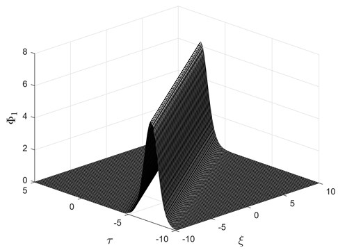
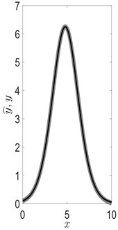
As follows from the previous subsection 3.1 (Eqs. (24)), (27) admits the following soliton solution:

if and only if initial conditions $u$, $v$ of Eq. (27) do satisfy the following constraint:

Soliton solution Eq. (28) is depicted in Fig. 1.

Returning to the original PDE (25), the soliton solution reads:

Fig. 1Soliton solution Eqs. (28) to (27) for u=110, v=150-101250

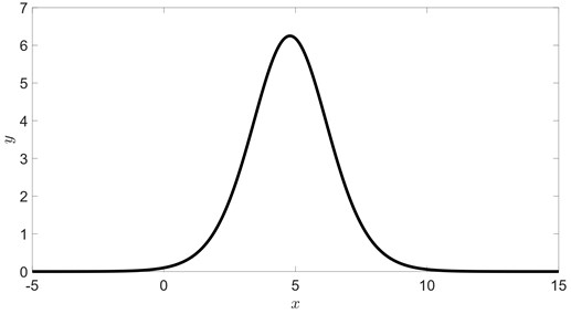
This solution is depicted in Fig. 2.

Fig. 2Soliton solution Eqs. (30) to (25) for u=110, v=150-101250

Constraint Eq. (29), ensuring that the solution to Eq. (27) has soliton form Eq. (28), can be illustrated via numerical integration. The error between analytical soliton solution Eq. (28) and the approximate solution to Eq. (27) (denoted as $\widehat{y}(x,x_0,u,v)$) is estimated using a constant-step, time-forward integrator as follows:

where $h$ denotes the integration step-size; $N$ is the number of integration steps. If soliton solution Eq. (28) to Eq. (27) would hold for all initial conditions $(x_0,u,v)$, then the error $\mathrm{\Delta }(x_0,u,v)$ would be zero for any $(x_0,u,v)$. However, Figs. 3, 4 demonstrate that this is not the case since the errors are close to zero only on the curve defined by Eq. (29).

Fig. 3The surface plot of the error Δ=Δ(x0,u,v) between Eq. (28) and the numerical solution to Eq. (27) for 0≤u≤6.5, -10≤v≤10. The error is evaluated using the step-size h= 0.01 and N= 100 time-forward steps. Errors higher than 5 are truncated to 5 for clarity. Note that the error is close to zero only on the curve defined by Eq. (29)

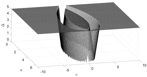
Fig. 4Black line in part (a) depicts the constraint Eq. (29), gray circle and gray diamond correspond to initial conditions (u,v) used in parts (b) and (c) respectively. Gray line in parts (b) and (c) displays an approximate solution to Eq. (27) (y^=y^(x,x0,u,v)), black line - analytical soliton solution Eq. (28) (y=y(x,x0,u,v)). It can be seen (part (b)) that approximate solution y^ and y coincide if initial condition (u,v) lies on the curve defined by Eq. (29). Otherwise, y^ and y are different (part (c))

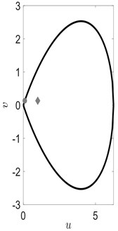
a)

b)

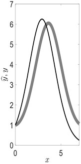
c)

5. Conclusions

Soliton solutions to Schamel equation considered in [1] are constructed using the concept of narrowed and extended differential equations. Necessary and sufficient conditions for the existence of these solutions have been derived in the space of equation parameters and initial conditions.

References

-
S. A. Shan, “Dissipative electron-acoustic solitons in a cold electron beam plasma with superthermal trapped electrons,” Astrophysics and Space Science, Vol. 364, No. 2, Feb. 2019, https://doi.org/10.1007/s10509-019-3524-1
H. Schamel, “A modified Korteweg-de Vries equation for ion acoustic wavess due to resonant electrons,” Journal of Plasma Physics, Vol. 9, No. 3, pp. 377–387, Jun. 1973, https://doi.org/10.1017/s002237780000756x
Z. Navickas, M. Ragulskis, and L. Bikulciene, “Be careful with the Exp-function method – Additional remarks,” Communications in Nonlinear Science and Numerical Simulation, Vol. 15, No. 12, pp. 3874–3886, Dec. 2010, https://doi.org/10.1016/j.cnsns.2010.01.032
Z. Navickas, L. Bikulciene, M. Rahula, and M. Ragulskis, “Algebraic operator method for the construction of solitary solutions to nonlinear differential equations,” Communications in Nonlinear Science and Numerical Simulation, Vol. 18, No. 6, pp. 1374–1389, Jun. 2013, https://doi.org/10.1016/j.cnsns.2012.10.009
About this article
The authors have not disclosed any funding.
The datasets generated during and/or analyzed during the current study are available from the corresponding author on reasonable request.
The authors declare that they have no conflict of interest.