Improving piano music signal recognition through enhanced frequency domain analysis

Gao, Hongjiao

doi:10.21595/jme.2024.23774

Journal of Measurements in Engineering

Browse Journal

Submit article

Published: 23 February 2024

Check for updates

Improving piano music signal recognition through enhanced frequency domain analysis

Hongjiao Gao¹

¹Music Department, Xinzhou Normal University, Xinzhou, Shanxi, 034000, China

Cite the article Download PDF

Article in Press

Downloads 42

Abstract

Feature extraction is a crucial component in the analysis of piano music signals. This article introduced three methods for feature extraction based on frequency domain analysis, namely short-time Fourier transform (STFT), linear predictive cepstral coefficient (LPCC), and Mel-frequency cepstral coefficient (MFCC). An improvement was then made to the MFCC. The inverse MFCC (IMFCC) was combined with mid-frequency MFCC (MidMFCC). The Fisher criterion was used to select the 12-order parameters with the maximum Fisher ratio, which were combined into the F-MFCC feature for recognizing 88 single piano notes through a support vector machine. The results indicated that when compared with the STFT and LPCC, the MFCC exhibited superior performance in recognizing piano music signals, with an accuracy rate of 78.03 % and an F1 value of 85.92 %. Nevertheless, the proposed F-MFCC achieved a remarkable accuracy rate of 90.91 %, representing a substantial improvement by 12.88 % over the MFCC alone. These findings provide evidence for the effectiveness of the designed F-MFCC feature for piano music signal recognition as well as its potential application in practical music signal analysis.

Improving piano music signal recognition through enhanced frequency domain analysis

Highlights

Several piano music signal features are introduced.
The feature screening is realized based on Fisher's criterion.
The performance of the extracted features is demonstrated by experimental comparison.

1. Introduction

With the continuous development of computer technology, music can be stored and produced through computers [1], making analysis and processing of music more convenient. Compared with speech signals, music signals have a richer timbre and more complex frequency variations. Therefore, the analysis and processing methods for speech signals are not completely applicable to music signals. The analysis and processing of music signals can provide support for tasks such as music information retrieval and music genre classification, making it a highly important research direction in the field of music [2]. Numerous methods have already been applied [3], such as deep learning (DL) [4], convolutional neural network [5], and deep neural network [6]. Li et al. [7] designed a supervised robust non-negative matrix factorization method to enhance the separation performance of instrumental music signals, such as piano and trombone. Experimental results demonstrated that this method yielded better separation effects compared to traditional approaches. Waghmare et al. [8] conducted a study on the classification and labeling of Indian music, proposed that Mel-frequency cepstral coefficients (MFCCs) can provide timbre information, and demonstrated the effectiveness of this method through experimental analysis. O'Brien et al. [9] conducted a study on the transcription of polyphonic music and proposed a probabilistic latent component analysis model. Their experiments demonstrated that this method effectively decomposed the signal into distinct hierarchical smooth structures, resulting in high-quality transcriptions. Hashemi et al. [10] introduced a DL-based approach for separating Persian musical sources and found that it performed well in isolating two audio sources and can also be applied to various audio sources and the combinations of more than two audio sources. Feature extraction is an important step in music signal analysis, which can generally be divided into two types: time domain and frequency domain. The traditional approach to music signal processing often emphasizes temporal characteristics, whereas the piano, being a polyphonic instrument, presents more intricate musical signals and larger volumes of temporal data. Compared to time domain analysis, piano music has a smaller computational load and better expression of musical information in frequency domain analysis. Currently, there is a dearth of research on piano music signal recognition, and the applicability of conventional speech signal analysis methods in this context is also limited. Therefore, this paper focused on the signal of piano music and extracted its features through frequency domain analysis. Several different features in the frequency domain were compared, and an improved MFCC feature was designed. Taking the recognition of 88 single piano notes as an example, the performance of the extracted features in recognizing piano music signals was demonstrated. The features extracted by the proposed method effectively represents the information embedded in piano music signals and emphasize crucial details to enhance recognition accuracy. The research on feature extraction, rather than recognition algorithms, significantly contributes to improving the interpretability of features. It reduces feature dimensions while preserving essential musical information, thus alleviating the computational burden of subsequent recognition algorithms and enabling their adaptation to complex music signal environments. Consequently, this directly enhances system performance. This work provides a novel approach for analyzing and processing music signals and promotes further advancements in digital music. The proposed features can be applied to the signal recognition of other musical instruments, which in turn can be extended to the field of speech signal processing.

2. Frequency analysis-based feature extraction

In the analysis and processing tasks of music signals, feature extraction of music signals is required to provide services for the subsequent research. Time domain analysis, such as short-time energy and zero-crossing rate [11], involves a large amount of data in computation; therefore, frequency domain analysis is more commonly used in signal analysis.

(1) Short-time Fourier transform (STFT).

STFT is a common feature extraction method based on frequency domain analysis [12], widely used in audio signal processing. It analyzes the time-frequency distribution of local signals to obtain the patterns of amplitude variation in the signal. The calculation formula is:

1

F_{M} (ω) = \sum_{n = - \infty}^{+ \infty} x (n) w (n - m S) e^{- i ω t},

where $x (n)$ represents an input signal, $w (n)$ is a window function, $w (n - m)$ is a sliding window, and $S$ is the step length of Fourier transform.

(2) Linear predictive cepstral coefficient (LPCC).

LPCC is a feature based on linear predictive coefficients (LPC) [13], which has certain advantages in suppressing low-frequency and high-frequency noise. It is assumed that after the LPC analysis of signal $x (n)$ , the obtained system transfer function is written as:

2

H (z) = \frac{1}{1 - \sum_{i = 1}^{p} a_{i} z^{- i}},

where $p$ denotes the model order and $a_{i}$ is a real number. A $p$ -order linear predictor is defined as:

3

F (z) = \sum_{i = 1}^{p} a_{i} z^{- i} .

The current sample is predicted using the first $p$ samples. The predictive value is:

4

\hat{x} (n) = \sum_{i = 1}^{p} a_{i} x (n - i) .

Then, the error function is obtained: $e (n) = x (n) - \hat{x} (n)$ . Coefficient $a_{i}$ that minimizes the mean square prediction error is known as the LPC.

After obtaining $a_{i}$ , the cepstrum is obtained by using the following recursion formula:

5

C_{i} = a_{i} + \sum_{k = 1}^{i = 1} (1 - \frac{k}{i}) C_{i - k} a_{k},

where $C_{i}$ is the LPCC.

(3) Mel-frequency cepstral coefficient (MFCC).

MFCC is a feature that references the characteristics of human auditory perception [14]. The relationship between Mel frequency and linear frequency $f$ is written as:

6

M e l (f) = 2595 * \log_{10} (1 + \frac{f}{700}) .

The preprocessed time-domain signal $x (n)$ is transformed to the frequency domain through fast Fourier transform (FFT):

7

X (k) = \sum_{n = 0}^{N - 1} x (n) e^{\frac{- 2 j n k π}{N}},

where $N$ stands for the number of points in Fourier transform. Then, the spectrum is smoothed through $M$ triangular bandpass filters to obtain output response $H_{m} (k)$ . The energy output of every filter is calculated, and the logarithm is taken. Then:

8

S (m) = \ln (\sum_{k = 0}^{n - 1} {|X (k)|}^{2} H_{m} (k)) .

Discrete cosine transform (DCT) is performed on $S (m)$ to obtain MFCC:

9

C_{i} = \sum_{k = 1}^{p} \log (S (m) \cos [i (k - \frac{1}{2}) \frac{π}{p}]),

where $i$ stands for the order of MFCC.

However, MFCC has a poor ability to extract information from mid and high-frequency audio. To address this issue, improvements need to be made to the coefficients of MFCC. Firstly, the high-frequency region of MFCC can be achieved through a reversed filter bank structure known as inverse MFCC (IMFCC) [15]. The response of the reversed filters can be expressed as:

10

{\hat{H}}_{i} (k) = H_{p - i + 1} (\frac{N}{2} - k + 1),

where $p$ stands for the number of filters. The relationship between IMFCC and linear frequency $f$ is written as:

11

f_{I M F C C} = 2840.1 - 1127 * \ln (1 + \frac{8000 - f}{700}) .

The MFCC in the middle frequency region is referred to as mid-frequency MFCC (MidMFCC) according to literature [16]. The relationship between MidMFCC and linear frequency $f$ is written as:

12

f_{M i d M F C C} = \{\begin{matrix} 1420 - 533.2 \times \ln (1 + \frac{4000 - f}{300}), 0 \leq f \leq 4000, \\ 1420 + 533.2 \times \ln (1 + \frac{f - 4000}{300}), 4000 \leq f \leq 8000 . \end{matrix}

By combining MFCC, IMFCC, and MidMFCC together, it is possible to extract complete information about the high-frequency, mid-frequency, and low-frequency regions of piano audio. However, a simple combination would greatly increase the dimensionality of the features. For example, if each parameter is taken as 12 orders, the total would be 36 orders which are not conducive to subsequent recognition and analysis of piano audio. Therefore, in order to reduce feature dimensionality, this paper applies Fisher criterion [17] for selecting MFCC+IMFCC+MidMFCC.

Fisher criterion determines the information amount in the feature dimensionality through calculating Fisher ratio. The corresponding formulas are:

13

F_{f i s h e r} = \frac{σ_{b e t w e e n}}{σ_{w i t h i n}},

14

σ_{b e t w e e n} = \sum_{i = 1}^{N} {(m_{k}^{i} - m_{k})}^{2},

15

σ_{w i t h i n} = \sum_{i = 1}^{N} \frac{1}{n_{i}} \sum_{c \in w_{i}} {({c_{k}^{i} - m}_{k}^{i})}^{2},

where $σ_{b e t w e e n}$ refers to the between-class distance, $σ_{w i t h i n}$ is the inner-class distance, $w_{i}$ refers to the $i$ -th kind of piano audio feature sequence, $m_{k}^{i}$ refers to the average value of the feature parameter of the $i$ -th kind of piano audio on the $k$ -th dimension, $m_{k}$ refers to the mean value of the $k$ -th dimensional feature on all classes, and $c_{k}^{i}$ is the $k$ -th component of the $i$ -th kind of piano audio feature sequence.

The Fisher ratio of MFCC, IMFCC, and MidMFCC is calculated, and the results are presented in Fig. 1.

The top 12 dimensions with the largest Fisher ratio in Fig. 1 are extracted as features for subsequent piano music recognition. For MFCC, the chosen orders include 1, 4, 5, 6, 7, and 10. For IMFCC, the chosen orders include 5, 6, and 9. For MidMFCC, the chosen orders include 6, 7, and 8.

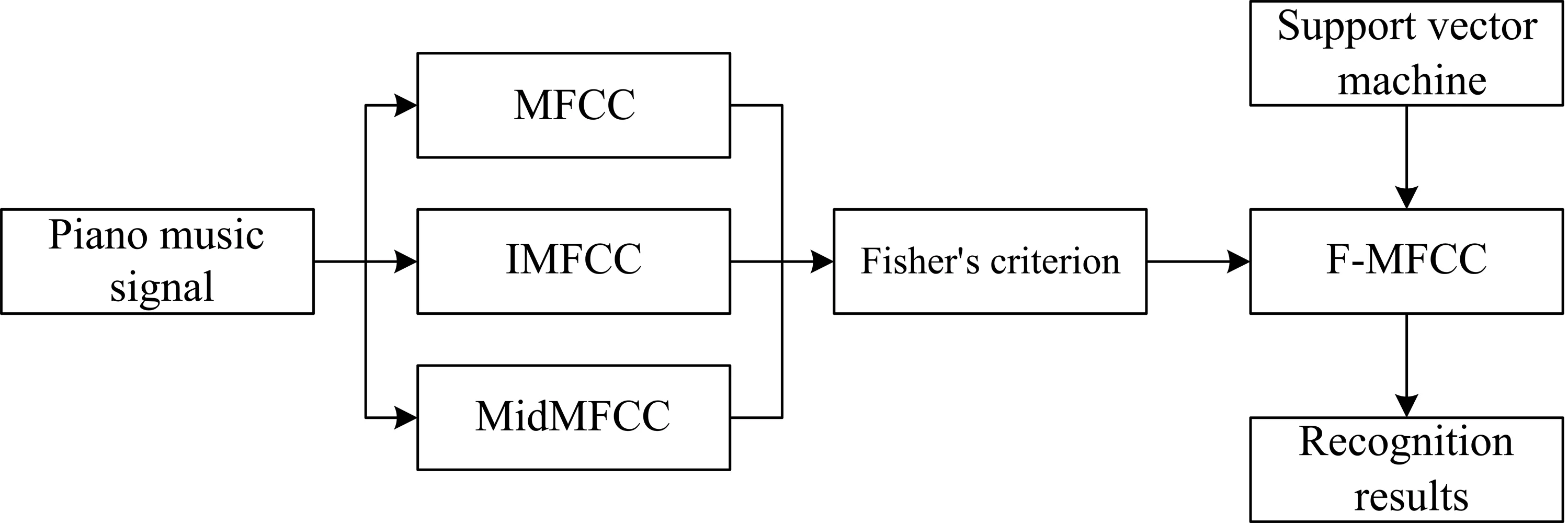
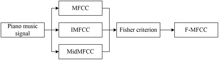
The features extracted by Fisher criterion are referred to as F-MFCC. The process of extracting F-MFCC is illustrated in Fig. 2.

After 12 orders of MFCC, IMFCC, and MidMFCC are extracted from the piano music signal, 12 orders of feature dimension with the largest Fisher ratio are selected using the Fisher criterion to obtain F-MFCC as the feature input of the subsequent piano music signal recognition.

3. Piano music signal recognition method

For the recognition of piano music signals, this paper employs the support vector machine (SVM) method. SVM is a statistical learning-based approach that offers effective solutions for nonlinearity and dimensionality curse problems [18]. It has a simple structure and has high flexibility [19]. It has been widely utilized in image classification, data prediction, and other domains [20]. It is assumed that there is linearly separable sample set $(x_{i}, y_{i})$ , $i = 1,2, \dots, n$ , $y \in \{+ 1, - 1\}$ . The equation of the classification plane can be written as: $w x + b = 0$ , satisfying:

16

y_{i} (w x_{i} + b) - 1 \geq 0 .

Fig. 1The Fisher ratio of MFCC, IMFCC, and MidMFCC

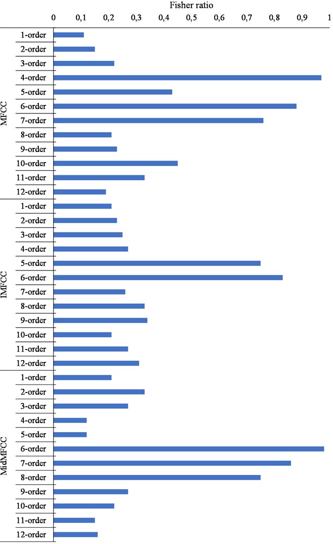
Fig. 2The extraction flow of F-MFCC

Moreover, the classification plane that minimize $\frac{1}{2} {‖w‖}^{2}$ is optimal. The Lagrange function is defined:

17

L (w, b, a) = \frac{1}{2} (w ∙ w) - \sum_{i = 1}^{n} a_{i} \{y_{i} (w x_{i} + b) - 1\},

where $a_{i}$ is a Lagrange coefficient. By setting the derivatives of $w$ and $b$ to zero, the original problem can be transformed into a dual problem. Under the condition of $\sum_{i = 1}^{n} y_{i} a_{i} = 0$ , $a_{i} \geq 0$ , the following equation is solved:

18

\max_{a} \sum_{i = 1}^{n} a_{i} - \frac{1}{2} \sum_{i, j = 1}^{n} a_{i} a_{j} y_{i} y_{j} (x_{i} ∙ x_{j}) .

If there is optimal solution $a_{i}^{*}$ , then $a_{i}^{*}$ .

The optimal classification function is written as: $f (x) = s g n \{\sum_{i = 1}^{n} a_{i}^{*} y_{i} (x_{i} ∙ x) + b^{*}\}$ .

In the selection of the kernel function, the Gaussian kernel function is used: $K (x_{i}, x_{j}) = e x p ({‖x_{i} - x_{j}‖}^{2} / σ^{2})$ , where $σ$ refers to the kernel function parameter.

4. Result and analysis

Eighty-weight single-tone data were collected from a regular piano, with a sampling rate of 44,100 Hz and a sampling time of 5 s. A total of ten sets was recorded, resulting in 880 samples. The collected data were saved in .wav format, allocating 70 % for the training set and 30 % for the test set. In the SVM, the parameter of the kernel function was determined through grid search and ultimately set to 0.5.

Table 1Confusion matrix

		Recognition results
		Positive sample	Negative sample
Actual results	Positive sample	TP	FN
Actual results	Negative sample	FP	TN

The recognition performance of different features was evaluated based on the confusion matrix (Table 1), with the following evaluation indicators. The final results were obtained by averaging the results from the 88 single-tones:

19

A c c u r a c y = \frac{T P + T N}{T P + F P + F N + T N},

20

R e c a l l = \frac{T P}{T P + F N},

21

P r e c i s i o n = \frac{T P}{T P + F P},

22

F 1 = \frac{2 \times P r e c i s i o n \times R e c a l l}{P r e c i s i o n + R e c a l l} .

Table 2 shows the recognition accuracy of the SVM method for the training set.

Table 2The recognition accuracy of the SVM method for the training set

Number of experiment	Recognition accuracy / %
1	89.26
2	90.12
3	90.15
4	90.13
5	89.87
6	89.92
7	90.77
8	89.65
9	90.81
10	89.97
Average value	90.0657

From Table 2, it can be observed that in the ten experiments, the SVM method achieved a recognition accuracy of approximately 90 % on the training set, with an average value of 90.07 %. This result indicated that the SVM method exhibited excellent precision in recognizing the training set.

Firstly, the impact of feature dimensionality selected by Fisher’s criterion on recognition accuracy was analyzed using the test set. The results are presented in Table 3.

Table 3The impact of the feature dimensionality selected by Fisher’s criterion on the recognition accuracy

	Recognition accuracy / %
6	87.64
12	90.91
18	77.33
24	71.25

From Table 3, it can be observed that an accuracy of 87.64 % was achieved when selecting the top 6-dimensional feature based on Fisher ratio as input. When choosing the top 12-dimensional feature based on Fisher ratio, the accuracy increased to 90.91 %, showing a significant improvement of 3.27 % compared to the case with only the 6-dimensional feature. However, as the dimensionality continued to increase, the accuracy gradually declined. Therefore, in subsequent experiments, the top 12-dimensional feature based on Fisher ratio was selected as F-MFCC and input into the SVM method for recognition.

A comparison was made among three frequency domain analysis methods: STFT, LPCC, and MFCC, using the test set. They all used the SVM method to recognize the 88 piano single-tone signals, and the results are presented in Table 4.

Table 4Recognition results of the SFTF, LPCC, and MFCC

		Actual result
		Positive sample	Negative sample
Recognition result of STFT	Positive sample	121	57
Recognition result of STFT	Negative sample	51	35
Recognition result of LPCC	Positive sample	145	24
Recognition result of LPCC	Negative sample	44	51
Recognition result of MFCC	Positive sample	177	21
Recognition result of MFCC	Negative sample	37	29

According to the results in Table 4, the recognition performance of the STFT, LPCC, and MFCC was calculated and presented in Table 5.

Table 5Comparison of the recognition performance between the STFT, LPCC, and MFCC

	STFT	LPCC	MFCC
Accuracy	59.09 %	74.24 %	78.03 %
Recall	70.35 %	76.72 %	82.71 %
Precision	67.98 %	85.80 %	89.39 %
F1	69.14 %	81.01 %	85.92 %

From Table 5, it can be observed that among the three frequency domain analysis-based features, the STFT performed the worst in recognizing piano music signals, with an accuracy rate of only 59.09 % and an F1 value of 69.14 %. When using LPCC as the feature input for the SVM method, the accuracy rate for recognizing piano single-tone signals reached 74.24 %, which showed a significant improvement of 15.15 % compared to the STFT. The F1value also increased to 81.01 %, showing an improvement of 11.87 % compared to the STFT. Compared to the STFT and LFCC, the MFCC achieved an accuracy rate of 78.03 % in single-tone recognition, which indicated a 3.79 % improvement over the LFCC. The recall rate and precision of the MFCC were 82.71 % and 89.39 %, respectively, both higher than those of the STFT and LFCC. The F1 value was 85.92 %, showing a significant increase of 4.91 % compared to the LFCC. These results indicated that among the three frequency domain features compared, the MFCC performed the best in recognizing piano music signals.

Then, the MFCC feature was further analyzed. The recognition results of the MFCC, IMFCC, and MidMFCC were compared (Table 6).

Table 6Recognition results of the MFCC, IMFCC, and MidMFCC

		Actual result
		Positive sample	Negative sample
Recognition result of MFCC	Positive sample	177	37
Recognition result of MFCC	Positive sample	21	29
Recognition result of IMFCC	Positive sample	170	37
Recognition result of IMFCC	Positive sample	27	30
Recognition result of MidMFCC	Positive sample	173	35
Recognition result of MidMFCC	Positive sample	24	32

According to Table 6, the recognition performance of the MFCC, IMFCC, and MidMFCC was calculated, and the results are shown in Table 7.

Table 7Comparison of recognition performance between the MFCC, IMFCC, and MidMFCC

	MFCC	IMFCC	MidMFCC
Accuracy	78.03 %	75.76 %	77.65 %
Recall	82.71 %	82.13 %	83.17 %
Precision	89.39 %	86.29 %	87.82 %
F1	85.92 %	84.16 %	85.43 %

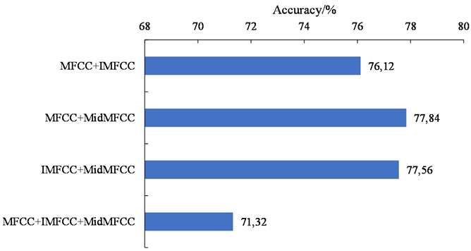
From Table 7, it can be observed that compared to the MFCC, IMFF and MidMFCC contained less information as they were based on the recomputation of the MFCC. Therefore, when used alone, their recognition performance was inferior to the MFCC. The F1 values of the IMFF and MidMFCC were 84.16 % and 85.43 %, respectively, both lower than that of the MFCC. The accuracy comparison between different combinations of the MFCC, IMFCC, and MidMFCC is shown in Fig. 3.

According to Fig. 3, when the MFCC, IMFCC, and MidMFCC were combined pairwise, there was no significant improvement in recognition accuracy compared to the MFCC. When all three features (MFCC+IMFCC+MidMFCC) were used as input for the SVM, the recognition accuracy dropped to 71.32 %, showing a decrease of 6.71 % compared to using only MFCC. The results demonstrated that an excessive number of feature dimensions could result in a decrease in recognition performance.

Fig. 3The accuracy of piano music signal recognition using different MFCC features

The F-MFCC was used as the SVM input and compared with the MFCC. The results of piano music signal recognition is shown in Fig. 4.

Fig. 4The performance of F-MFCC in piano music signal recognition

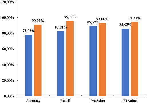
From Fig. 4, it can be observed that when using the F-MFCC as the feature, the SVM demonstrated a significant improvement in recognizing piano music signals. Firstly, in terms of the accuracy, the F-MFCC achieved 90.91 %, which represented an increase of 12.88 % compared to the MFCC; secondly, in terms of the recall rate, the F-MFCC achieved 95.71 %, indicating a 13 % increase compared to the MFCC. The F-MFCC achieved a precision of 93.06 %, which was a 3.67 % improvement compared to the MFCC. In terms of the F1 value, the F-MFCC achieved 94.37 %, which was a 8.45 % improvement compared to the MFCC. The F-MFCC selected 12-order MFCC parameters with the highest information content and combined them as the feature input for the SVM, thereby achieving improved performance in recognizing piano music signals.

The accuracy of piano music signal recognition was evaluated as an example. Ten-fold cross-validation was performed to obtain ten accuracy values, which were then averaged. A t-test was conducted to compare the accuracy of the F-MFCC with the other features, and the $p$ value was computed. If $p <$ 0.05, it indicated a significant difference between the F-MFCC and the other features. The results are presented in Table 8.

Table 8Statistical analysis of recognition accuracy

	Accuracy	$p$ value
F-MFCC	90.33±0.89	–
STFT	59.35±2.26	< 0.001
LPCC	75.12±1.16	0.016
MFCC	79.84±1.34	0.017
IMFCC	76.77±2.07	0.021
MidMFCC	77.81±1.16	0.018
MFCC+IMFCC	78.12±1.25	0.036
MFCC+MidMFCC	79.33±1.33	0.019
IMFCC+MidMFCC	78.56±1.27	0.022
MFCC+IMFCC+MidMFCC	72.33±2.08	0.027

The recognition accuracy of the other features was lower compared to the F-MFCC, as observed from Table 8. Through comparison, it can be concluded that there was a significant difference between the accuracy obtained from the F-MFCC and other features ( $p <$ 0.05). This result demonstrated the distinct advantage of the F-MFCC in piano music signal recognition.

5. Discussion

Music signal processing has extensive practical applications, such as audio content recognition and analysis, as well as the enhancement and noise reduction of audio. In the field of music composition, based on music signal processing, it is possible to synthesize virtual instruments and achieve automated note and melody recognition, thereby enhancing the intelligence of music creation. Feature extraction plays a crucial role in music signal processing as it directly affects the recognition and classification results of musical signals. Therefore, this paper focuses on improving piano music signal recognition effectiveness through improved frequency domain analysis.

MFCC is a commonly used feature in signal processing. This paper further enhanced the extraction of piano audio features by incorporating IMFCC and MidMFCC based on MFCC. Subsequently, Fisher's criterion was applied to filter the obtained features, resulting in the F-MFCC feature. Through the recognition experiment on 88 individual piano notes, it can be observed that compared to the STFT and LPCC, the MFCC exhibited better performance in recognizing piano music signals. MFCC is a feature that aligns more closely with human auditory characteristics, thus the SVM method based on MFCC achieved higher accuracy in single note recognition, thus proving the reliability of selecting MFCC for further research.

When comparing the MFCC, IMFCC, and MidMFCC, it can be observed that both IMFCC and MidMFCC did not perform as well as MFCC in single-tone recognition. Additionally, when combined pairwise, they also did not achieve higher recognition accuracy. Surprisingly, when all 36-dimensional features of the MFCC, IMFCC, and MidMFCC were used as inputs for SVM classification, the obtained accuracy actually decreased. This suggested that an excessive number of dimensions led to a decrease in precision. The F-MFCC features selected by the Fisher criterion achieved the highest recognition accuracy, i.e., 90.91 %. This represented a 12.88 % improvement compared to the MFCC and demonstrated both the reliability of the designed F-MFCC as a feature for piano music signal recognition and its potential for further application in practical music signal processing.

6. Conclusions

This article conducted a study on the extraction of piano music signal features from the perspective of frequency domain analysis. A Fisher criterion-based F-MFCC feature was designed, and the SVM was used to recognize 88 single piano notes. From the results, it can be observed that the STFT and LPCC exhibited poor performance in recognizing piano music signals. The accuracy and F1 value of the MFCC were found to be 78.03 % and 85.92 %, respectively, which were superior to those of the STFT and LPCC. When comparing different MFCC features, it can be observed that an excessive number of feature parameters led to a decrease in recognition performance. However, the proposed F-MFCC achieved an accuracy of 90.91 % and an F1 score of 94.37 %, demonstrating significant improvements compared to the MFCC. The findings highlight the effectiveness of the proposed method and its potential for practical applications. However, this study also has some limitations. For example, it solely focuses on extracting piano music signal features while overlooking the optimization of recognition algorithms. Additionally, the size of the experimental data was relatively small. In future work, we will make further improvements and optimizations to the SVM method and conduct experiments on a wider range of data to validate the reliability of the proposed approach.

References

M. Goto and R. B. Dannenberg, “Music interfaces based on automatic music signal analysis: new ways to create and listen to music,” IEEE Signal Processing Magazine, Vol. 36, No. 1, pp. 74–81, Jan. 2019, https://doi.org/10.1109/msp.2018.2874360

Publisher
M. Müller, B. McFee, and K. M. Kinnaird, “Interactive learning of signal processing through music,” IEEE Signal Processing Magazine, Vol. 38, No. 3, pp. 73–84, 2021.

Publisher
M. Mueller, B. A. Pardo, G. J. Mysore, and V. Valimaki, “Recent advances in music signal processing,” IEEE Signal Processing Magazine, Vol. 36, No. 1, pp. 17–19, Jan. 2019, https://doi.org/10.1109/msp.2018.2876190

Publisher
W. Feng, J. Liu, T. Li, Z. Yang, and D. Wu, “FAC: a music recommendation model based on fusing audio and chord features (115),” International Journal of Software Engineering and Knowledge Engineering, Vol. 32, No. 11n12, pp. 1753–1770, Oct. 2022, https://doi.org/10.1142/s0218194022500577

Publisher
X. Fu, H. Deng, and J. Hu, “Automatic label calibration for singing annotation using fully convolutional neural network,” IEEJ Transactions on Electrical and Electronic Engineering, Vol. 18, No. 6, pp. 945–952, Apr. 2023, https://doi.org/10.1002/tee.23804

Publisher
D. Schneider, N. Korfhage, M. Mühling, P. Lüttig, and B. Freisleben, “Automatic transcription of organ tablature music notation with deep neural networks,” Transactions of the International Society for Music Information Retrieval, Vol. 4, No. 1, pp. 14–28, Feb. 2021, https://doi.org/10.5334/tismir.77

Publisher
F. Li and H. Chang, “Music signal separation using supervised robust non-negative matrix factorization with β-divergence,” International Journal of Circuits, Systems and Signal Processing, Vol. 15, pp. 149–154, Feb. 2021, https://doi.org/10.46300/9106.2021.15.16

Publisher
K. C. Waghmare and B. A. Sonkamble, “Analyzing acoustics of Indian music audio signal using timbre and pitch features for raga identification,” in 2019 3rd International Conference on Imaging, Signal Processing and Communication (ICISPC), pp. 42–46, Jul. 2019, https://doi.org/10.1109/icispc.2019.8935707

Publisher
C. Obrien and M. D. Plumbley, “A hierarchical latent mixture model for polyphonic music analysis,” in 2018 26th European Signal Processing Conference (EUSIPCO), pp. 1910–1914, Sep. 2018, https://doi.org/10.23919/eusipco.2018.8553244

Publisher
S. S. Hashemi, M. Aghabozorgi, and M. T. Sadeghi, “Persian music source separation in audio-visual data using deep learning,” in 2020 6th Iranian Conference on Signal Processing and Intelligent Systems (ICSPIS), pp. 1–5, Dec. 2020, https://doi.org/10.1109/icspis51611.2020.9349614

Publisher
Y. W. Chit and S. S. Khaing, “Myanmar continuous speech recognition system using fuzzy logic classification in speech segmentation,” in ICIIT 2018: 2018 International Conference on Intelligent Information Technology, pp. 14–17, Feb. 2018, https://doi.org/10.1145/3193063.3193071

Publisher
Q. H. Pham, J. Antoni, A. Tahan, M. Gagnon, and C. Monette, “Simulation of non-Gaussian stochastic processes with prescribed rainflow cycle count using short-time Fourier transform,” Probabilistic Engineering Mechanics, Vol. 68, p. 103220, Apr. 2022, https://doi.org/10.1016/j.probengmech.2022.103220

Publisher
Y.-B. Wang, D.-G. Chang, S.-R. Qin, Y.-H. Fan, H.-B. Mu, and G.-J. Zhang, “Separating multi-source partial discharge signals using linear prediction analysis and isolation forest algorithm,” IEEE Transactions on Instrumentation and Measurement, Vol. 69, No. 6, pp. 2734–2742, Jun. 2020, https://doi.org/10.1109/tim.2019.2926688

Publisher
D. Taufik and N. Hanafiah, “AutoVAT: an automated visual acuity test using spoken digit recognition with Mel frequency cepstral coefficients and convolutional neural network,” Procedia Computer Science, Vol. 179, No. 4, pp. 458–467, Jan. 2021, https://doi.org/10.1016/j.procs.2021.01.029

Publisher
S. Chakroborty, A. Roy, S. Majumdar, and G. Saha, “Capturing complementary information via reversed filter bank and parallel implementation with MFCC for improved text-independent speaker identification,” in 2007 International Conference on Computing: Theory and Applications (ICCTA’07), pp. 463–467, Mar. 2007, https://doi.org/10.1109/iccta.2007.35

Publisher
J. Zhou, G. Wang, Y. Yang, and P. Chen, “Speech emotion recognition based on rough set and SVM,” 2006 5th IEEE International Conference on Cognitive Informatics, Vol. 20, No. 5, pp. 597–602, Jul. 2006, https://doi.org/10.1109/coginf.2006.365676

Publisher
S. J. Sree, “Analysis of lung CT images based on fisher criterion and genetic optimization,” IARJSET, Vol. 6, No. 3, pp. 36–41, Mar. 2019, https://doi.org/10.17148/iarjset.2019.6307

Publisher
C. Singh, E. Walia, and K. P. Kaur, “Enhancing color image retrieval performance with feature fusion and non-linear support vector machine classifier,” Optik, Vol. 158, pp. 127–141, Apr. 2018, https://doi.org/10.1016/j.ijleo.2017.11.202

Publisher
Y. Zhao, “Precision local anomaly positioning technology for large complex electromechanical systems,” Journal of Measurements in Engineering, Vol. 11, No. 4, pp. 373–387, Dec. 2023, https://doi.org/10.21595/jme.2023.23319

Publisher
Q. Chen and Y. Huang, “Prediction of comprehensive dynamic performance for probability screen based on AR model-box dimension,” Journal of Measurements in Engineering, Vol. 11, No. 4, pp. 525–535, Dec. 2023, https://doi.org/10.21595/jme.2023.23522

Publisher

About this article

Received

06 November 2023

Accepted

26 January 2024

Published

23 February 2024

DOI

https://doi.org/10.21595/jme.2024.23774

Keywords

frequency domain analysis

piano

music signal

feature extraction

Acknowledgements

The authors have not disclosed any funding.

Data Availability

The datasets generated during and/or analyzed during the current study are available from the corresponding author on reasonable request.

Conflict of interest

The authors declare that they have no conflict of interest.

This is an open access article distributed under the Creative Commons Attribution License, which permits unrestricted use, distribution, and reproduction in any medium, provided the original work is properly cited.

Research article

2023 10 31

Research on tool condition monitoring (TCM) using a novel unsupervised deep neural network (DNN)

Jingjing Gao, Jing Liu, Xinli Yu

Research article

2023 03 13

Extraction and recognition of music melody features using a deep neural network

Zhongqing Zhang

Review article

2022 06 26

Recent advancements of signal processing and artificial intelligence in the fault detection of rolling element bearings: a review

A. Anwarsha, T. Narendiranath Babu

Review article

2021 11 26

Fault diagnosis and health management of bearings in rotating equipment based on vibration analysis – a review

Adnan Althubaiti, Faris Elasha, Joao Amaral Teixeira

H. Gao, “Improving piano music signal recognition through enhanced frequency domain analysis,” Journal of Measurements in Engineering, Vol. 12, No. 2, –11, Feb. 2024, https://doi.org/10.21595/jme.2024.23774

Copy Extrica

Copied to clipboard!

TY  - JOUR
DO  - 10.21595/jme.2024.23774
UR  - https://doi.org/10.21595/jme.2024.23774
TI  - Improving piano music signal recognition through enhanced frequency domain analysis
T2  - Journal of Measurements in Engineering
AU  - Gao, Hongjiao
PY  - 2024
DA  - 2024/02/23
PB  - Extrica
VL  - 12
IS  - 2
SN  - 2335-2124
SN  - 2424-4635
ER  - 

Copy Ris

Copied to clipboard!

 @article{Gao_2024, title={Improving piano music signal recognition through enhanced frequency domain analysis}, ISSN={2424-4635}, url={https://doi.org/10.21595/jme.2024.23774}, DOI={10.21595/jme.2024.23774}, journal={Journal of Measurements in Engineering}, publisher={JVE International Ltd.}, author={Gao, Hongjiao}, year={2024}, month=feb }

Copy Bibtex

Copied to clipboard!

[1]H. Gao, “Improving piano music signal recognition through enhanced frequency domain analysis,” Journal of Measurements in Engineering, Feb. 2024, doi: 10.21595/jme.2024.23774.

Copy IEEE

Copied to clipboard!

Gao, Hongjiao. “Improving Piano Music Signal Recognition through Enhanced Frequency Domain Analysis.” Journal of Measurements in Engineering, February 23, 2024. https://doi.org/10.21595/jme.2024.23774.

Copy Chicago

Copied to clipboard!

Improving piano music signal recognition through enhanced frequency domain analysis

Abstract

Highlights

1. Introduction

2. Frequency analysis-based feature extraction

3. Piano music signal recognition method

4. Result and analysis

5. Discussion

6. Conclusions

References

About this article

Related Articles