Abstract
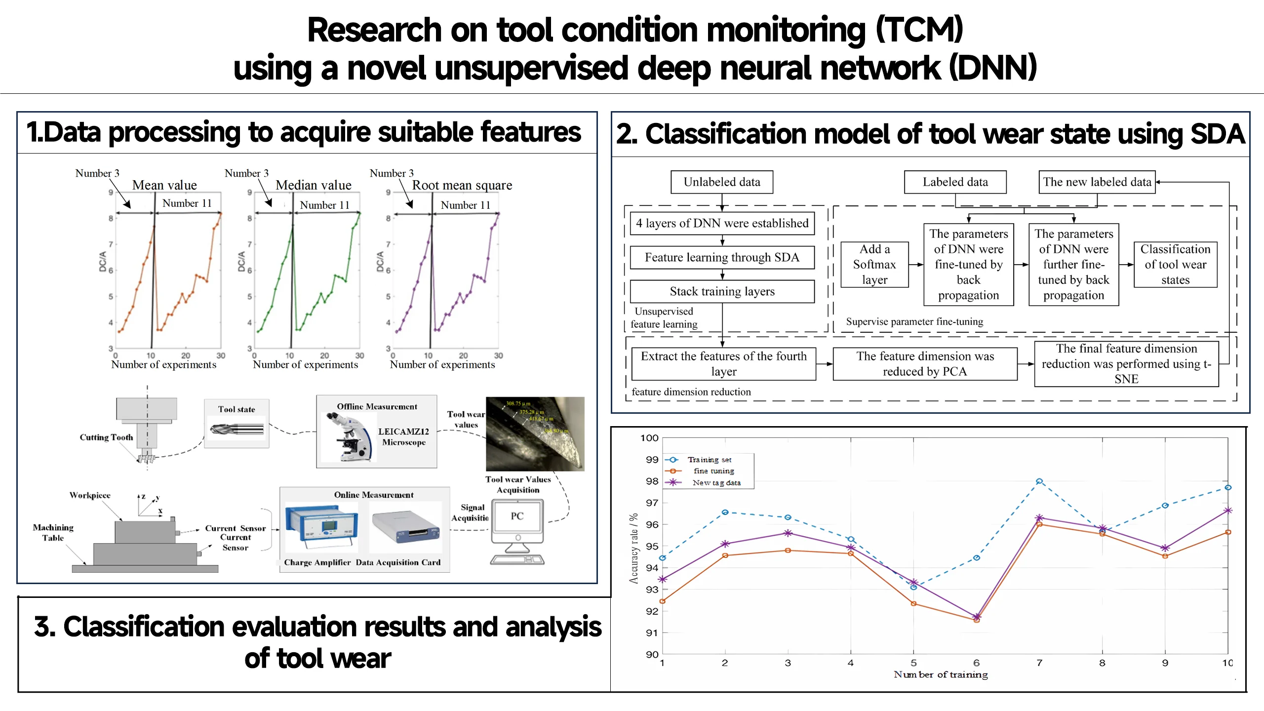
In order to improve the recognition precision and accuracy of tool wear monitoring, an unsupervised deep neural network (DNN) based on stack denoising autoencoder (SDA) is proposed. After feature extraction and selection, the stack denoising automatic coding network reduces the dimensionality of the feature vector. On this basis, principal component analysis (PCA) and T-distributed random neighbor embedding (t-SNE) are used to reduce the dimensionality of the features twice, and finally a simple two-dimensional feature matrix is obtained. Finally, the deep neural network model of SDA is established by adding SoftMax regression layer, and the tool wear monitoring results are taken as new labeled data, and the deep neural network parameters are fine-tuned by secondary backpropagation. The experimental results show that the proposed method can learn adaptively and obtain effective feature expression, and the tool wear state recognition results are highly accurate. The proposed method can effectively identify the tool wear state.
Highlights
- The feature matrix is preliminarily dimensionally reduced.
- The tool wear monitoring results were taken as the new labeled data.
- The deep neural network parameters were fine adjusted by secondary backpropagation.
1. Introduction
The material removal is realized under the interaction between the tool and the workpiece, and TCM is crucial to the machining process of the part. Therefore, it is necessary to identify and monitor the status of the tool, so as to make a reasonable tool change and ensure the processing quality and efficiency. Therefore, TCM is an important aspect of tool wear research.
The methods of TCM can be divided into direct monitoring and indirect monitoring. Direct monitoring is to use optical technology or machine vision technology to directly observe the TCM. The direct monitoring method usually uses the image analysis method to monitor the tool conditions.[1] The direct monitoring method does not affect the milling process and has higher recognition accuracy. However, when the monitoring process is affected by other factors, such as chips or cutting fluid sometimes remaining on the observed surface, it is difficult to ensure that the cutting wear state can be completely observed [2]. Therefore, this paper uses the indirect monitoring method to study the TCM. The indirect monitoring method is based on the measured signals in machining, then uses signal processing method and pattern recognition method to identify tool wear indirectly. The commonly used signal processing methods include time domain method, frequency domain method and time-frequency method. Common pattern recognition models include artificial neural network (ANN), hidden Markov model (HMM), support vector machine (SVM) and so on.
The choice of sensor directly determines the accuracy of signal and the reliability of recognition. Vibration sensor is extremely important and in the core position of the sensor [3, 4]. Commonly used vibration sensor types are displacement sensor, acceleration sensor, speed sensor, laser Doppler sensor and so on. Additionally, many scholars use cutting force signal to do TCM [5-7]. With the wear of the tool, the fillet radius of the cutting edge of the tool will continue to increase, resulting in the change of the cutting force. Therefore, cutting force is not only sensitive to tool wear status, but also can accurately reflect tool wear status with cutting. Cutting force can be reflected by spindle power or bending moment, so they can also be used to identify the degree of tool wear. As shown in Figure 1, bending moment is adopted to detect tool wear. However, force sensors are usually large and expensive, and their installation range is often limited [8].
Acoustic emission (AE) can also be used in TCM due to that it can realize their functions by detecting stress waves generated by local defects in materials [9, 10]. However, when the stress wave is transmitted between the media, its attenuation is relatively serious. Hence, the coupling agent is usually applied between the object to be measured and the sensor. AE will also be affected by multiple factors such as installation location, working mode and environmental noise [11].
TCM based on the machine tool built-in sensors such as current sensing overcomes the above limitations and is conducive to the promotion in industry. However, Luo Ming et al. [12] pointed out that the worn tool can be detected according to the relationship between the spindle power and the cutting force, but the specific blade cannot be identified.
It has been shown that if only one sensor is used, all the characteristics of tool wear status cannot be obtained, because each signal has different sensitivity to tool status changes [13]. Therefore, researchers usually collect signals from multiple sensors to detect tool wear, and have achieved significant results [14, 15]. However, in any of the above ways, the sensor needs to be reinstalled, and sometimes even the machine tool needs to be modified.
The data sets constructed from the collected signals are sometimes unbalanced. Data imbalance usually refers to differences in the amount of data in each category. There are many ways to solve the imbalance problem, such as getting more data, changing another judgment method, reorganizing the data, and so on. The over- sampling method is one of the methods of reorganizing data. The adaptive synthetic sampling method (ADASYN) is a simple and effective oversampling method [16].
When effective signals are obtained, a series of operations such as feature extraction, feature selection and feature dimension reduction are generally carried out by signal processing methods, Different signals and features have different sensitivity to tool wear. Therefore, it is sometimes necessary to adopt sensitivity analysis and determining the index of feature selection. After the feature is determined, a classifier model should be established to recognize tool wear. AI Azmi [7] found that the characteristic components associated with tool wear were mainly concentrated in the sixth-, seventh- and eighth-order components of LPCC. Karandikar et al. [17] described a naive Bayes classifier method for TCM. Liu et al. [18] verified that mechanistic cutting force model had the potential for monitoring micro-milling tool wear. A TCM system established by Seemuang et al. [19] can increase the competitiveness of a machining process by increasing the utilized tool life and decreasing instances of part damage from excessive tool wear or tool breakage. Tool wear and breakage is one of the biggest obstacles for developing the unattended CNC machining [20]. Scholars sometimes use multiple classifiers to identify tool wear. The final decision was made by fusion at the classifier level, and the tool wear identification was realized in Ref. [21].
With the development of data processing technology, information technology, sensing technology and so on, tool wear status and evaluation methods are constantly developing. In this paper, a TCM model based on the built- in sensors of machine tools is proposed. Since the data are derived from the built-in current sensors of machine tools, and no other sensors are needed, this model can be widely used in industrial CNC machine tools. Additionally, it can be seen that most literature focuses on manual feature extraction, and researchers pay little attention to the automatic feature extraction. Few scholars adopt an unsupervised learning methods to monitor the tool wear.
To solve above problems, a novel unsupervised DNN based on SDA is proposed in this paper. and classification of tool wear conditions. The rest of paper is organized as follows: in the first section, in order to find features that can characterize tool wear, systematic processing methods are conducted, including data preprocessing, feature extraction, feature selection, feature dimension reduction. Among them, time domain features, frequency domain features, time-frequency features are viewed as the original features. The selection of tool wear feature is based on the fact that the feature needs to have some correlation and monotonicity with tool wear. PCA and t-SNE are together adopted to reduce the feature dimension. The second part mainly introduce the classification of tool wear state. In order to complement the automatic identification, a DNN model based on SDA is proposed to realize the classification.
2. Data processing to acquire suitable features
2.1. Data acquisition
The experiment adopts MC-510V machining center to carry out multi-condition tool wear experiment. The experimental platform is shown in Fig. 1. In the end, 16 experiments were carried out under 8 working conditions, as shown in Table 1. We collect spindle motor current signal (AC), spindle motor current signal (DC), and the flank wear (VB).
Fig. 1Setup of the experimental platform
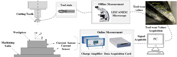
In the signal acquisition stage, according to the analysis of each sensor, the built-in sensor of the machine tool is suitable for normal production environment, overcoming the above limitations, and the current sensor is one of the common sensors. Therefore, this paper studies the monitoring and evaluation model of tool wear condition based on the built-in current sensor of machine tool. The current sensor is set on the test bench, and the collected signal is amplified and filtered, and collected to the terminal processor of the computer through two signal acquisition cards. The current signal of the spindle motor is directly connected to the computer terminal processor without any pre-processing steps. The current converter model is Omron K3TBA1015, which is used to change the AC current flow of the spindle into DC current and collect DC current. It is represented by “DC signal”. The model of the AC current sensor is CTA 213, and the collected signal is represented by “AC signal”.
The experiment used 3 factor 2 level full factor experiment. The cutting depth is 1.50 mm and 0.75 mm, the feed speed is 0.5 mm/r and 0.25 mm/r, and the workpiece material is cast iron and steel. The cutting speed is maintained at 200 m/min, and the corresponding spindle speed is 826 r/min. The length, width and height of the milling workpiece are 483 mm, 178 mm and 51 mm respectively. The cutter has a diameter of 70 mm and is embedded with 6 KC710 blades. The blade adopts TiC/TICN/TiN coating, which not only retains the toughness of tungsten carbide, but also improves the shrinkage resistance and reduces the grinding.
In this experiment, the sampling frequency is set to 250 Hz, that is, the sampling period is 0.8 ms. For each tool walking process, the signal acquisition time is 36 s, that is, the data sample length is 9000. Two repeated experiments were carried out for each operating parameter. In the end, 16 experiments were carried out under 8 working conditions, as shown in Table 1. In each group of experiments, a new tool was used to carry out repeated cutting experiments under the set operating conditions, and the VB value of the back tool face wear was measured at the end of each tool. When the VB value exceeds the threshold, the experiment ends and the next set of cutting parameters is tested. According to the literature method, all working conditions were grouped into six groups, as shown in Table 3.
Table 1Experimental parameters setup
Working condition | Cutting depth (mm) | Feed rate f (mm/min) | Workpiece material |
1 | 1.5 | 0.5 | Cast iron |
2 | 0.75 | 0.5 | Cast iron |
3 | 0.75 | 0.25 | Cast iron |
4 | 1.5 | 0.25 | Cast iron |
5 | 1.5 | 0.5 | Steel |
6 | 1.5 | 0.25 | Steel |
7 | 0.75 | 0.25 | Steel |
8 | 0.75 | 0.5 | Steel |
9 | 1.5 | 0.5 | Cast iron |
10 | 1.5 | 0.25 | Cast iron |
11 | 0.75 | 0.25 | Cast iron |
12 | 0.75 | 0.5 | Cast iron |
13 | 0.75 | 0.25 | Steel |
14 | 0.75 | 0.5 | Steel |
15 | 1.5 | 0.25 | Steel |
16 | 1.5 | 0.5 | Steel |
2.2. Data preprocessing
A total of 167 samples was collected in the form of a structured array of MATLAB files, in which the first 7 columns of the structured array are the experimental serial number of processing, the number of cutting times under each experimental serial number, and the measured tool flank wear after cutting (not measured after each cutting), cutting times (retimed for new working conditions), cutting depth, feed rate, workpiece material, and the last two columns are the DC and AC current signals measured from the built-in sensor of the spindle motor. The data obtained in the experiment is not intact, and there are some abnormal situations, resulting in data damage or loss. Before data analysis, the data needs to be preprocessed. The specific process is as follows:
(1) Delete abnormal sensor data. In the 18th run, the current signal was abnormal, and its data was far beyond the measurement range of the sensor. At the 95th run, the current signal is almost zero. These two records were outliers, they were removed before analysis, and then the rest of the samples were rearranged from 1 to 165 in order of experiment.
(2) Handle missing data. There are several samples whose VB values were missing, such as the 2nd and 3rd cutting experiments. Set the VB value of the tool's first cutting in each working condition to 0 and use spline interpolation to calculate the unknown VB value.
2.3. Construction of tool wear status indicator
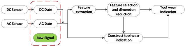
The real-time data obtained from the built-in current sensor of the machine tool contains information related to the wear state of the tool at each instant. In order to monitor the wear state of the tool, the original data needs to be further processed to find the characteristic matrix representing the wear state of the tool. To this end, it is necessary to start from three aspects as shown in Fig. 2: feature extraction, feature selection and dimensionality reduction, and construction of tool wear status indicators.
Fig. 2Construction flow of tool wear indicators
2.4. Feature extraction and selection
Feature extraction plays an important role in machine learning and data analysis. It can help us work with high-dimensional data, improve model performance, provide data visualization and understanding, and achieve goals such as interpretability and feature engineering. By selecting appropriate feature extraction methods and strategies, we can extract the most valuable and meaningful features from the original data, providing a better foundation for subsequent analysis and modeling.
For better feature extraction and selection, the DC and AC signals of the working condition group are compared with the VB value, and the working condition of group C is selected.
There is a great correlation between DC signal and AC signal and VB value of tool wear. Due to the equivalence effect (effective value) between AC signal and DC signal, and from the above figure, the correlation between DC signal and VB value is stronger, which is more consistent with the monotonic feature of the feature. Therefore, DC current signal is selected for feature extraction. However, the rising and falling stages are unstable stages, hence the stable stage is used as the original signal in feature extraction and selection.
2.5. Feature selection and dimension reduction
2.5.1. Feature selection
Feature selection can reduce the number of features, reduce dimension, make the model more generalization ability, reduce overfitting, and enhance the understanding between features and feature values.
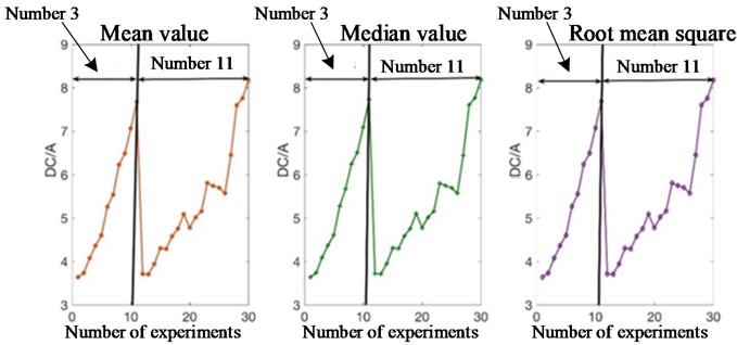
The selection of tool wear features is based on the fact that the features must have some correlation with the tool wear and have monotonicity. The feature mainly includes three aspects: time domain feature, frequency domain feature and time frequency feature. In the time domain features, statistical features whose variation trend is the same as that of tool wear amount are selected, as shown in Fig. 3. It is verified that the mean value, median value and root mean square of in the stable stage of DC signal are selected as the time-domain characteristics of tool wear.
The same rule is used to select the frequency domain features. After tool wear, the energy consumption will increase. The frequency band energy represents the amount of energy, which is calculated using the following equation:
where, is the spectrum amplitude of DC signal, and represents the value range of spectrum.
The median frequency can reflect the position change of the main frequency. When the tool wear increases, the median frequency will inevitably change along with it. The median frequency can be calculated using the following equation:
where, is the frequency of the spectrum, and is the sampling frequency.
With the increase of tool wear, the average energy of the signal increases, hence the mean square frequency can also reflect the change of tool wear. The mean square frequency can be calculated by the following equation:
Peak frequency represents the operating current frequency of the motor, and has a great correlation with tool wear, which can be calculated by the following equation:
Fig. 3Change of three-time domain features with the experiments
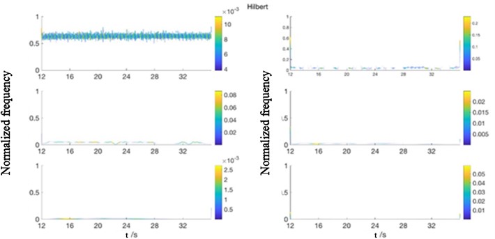
In time-frequency feature extraction, the signal is decomposed into different frequency bands by EMD, and then the Hilbert spectrum of each frequency band is obtained by Hilbert Huang Transform (HHT), as shown in Fig. 4 and Fig. 5. Figures shows the EMD decomposition of DC signal EMD decomposition. Then, the statistical features of the Hilbert spectrum are extracted, including the mean value, root mean square, kurtosis factor, skewness and other features. The calculation process of HHT is divided into two steps: first, the signal is decomposed by EMD; Then, in order to obtain the instantaneous frequency and amplitude of the original signal, HHT is performed on the IMF obtained by EMD. Let the analytical expression of IMF be, , which is defined by the following equation:
Among them is the IMF HHT, which is to say:
where, is Cauchy principal value. Using the extreme coordinates of the analytical expression of IMF, the instantaneous amplitude and phase can be calculated as follows:
Next, the instantaneous frequency can be derived from the instanta neous phase , which is expressed in the following equation:
Finally, the original signal can be expressed as follows:
where, Re is the real part of the signal and is the length of the signal. The HHT of signal is:
where, is the time-frequency distribution of the ith IMF of signal , and ) represents the function of the IMF amplitude and instantaneous frequency .
Fig. 4EMD decomposition of DC signal when 𝑎𝑟 = 0.75 mm, 𝑓 = 0.25 mm/r, 𝑉𝐵 = 0.40 mm
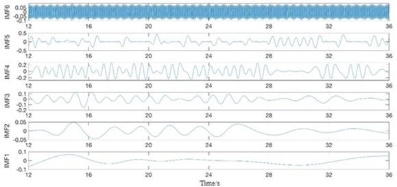
Fig. 5HHT spectrum of IMFs after EMD when 𝑎𝑟 = 0.75 mm, 𝑓 = 0.25 mm/r, 𝑉𝐵 = 0.40 mm
The selection rules of time domain and frequency domain features are adopted: the features with the same variation trend as tool wear are selected. By comparison, only the mean of the Hilbert spectrum of IMF1 is selected in the time-frequency features. The comparison between the variation trend and tool wear is shown in Fig. 4.
In summary, the total features of each signal in group c are composed of time domain (3 features), frequency domain (4 features), and time-frequency domain (1 feature), as shown in Table 2.
Fig. 6Comparison between HHT spectrum and tool wear of IMF1
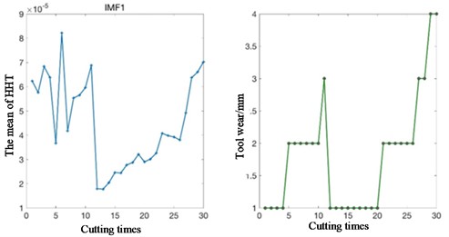
Table 2Total features of signal
Features in the domain | Characteristics of the |
The time domain | Original signal mean |
Median value of original signal | |
Root mean square of original signal | |
Frequency domain | The frequency domain energy |
The median frequency | |
The mean square frequency | |
Peak frequency | |
Time and frequency domain | Mean of the Hilbert spectrum of IMF1 |
2.5.2. Feature dimension reduction
Feature dimensionality reduction transforms high-dimensional data into low-dimensional data by removing redundant and irrelevant features, which is a beneficial data preprocessing step that can improve computational efficiency, eliminate redundant information, prevent overfitting, and help improve model interpretability and generalization ability.
In order to find a simple, automatic and intelligent feature extraction method, this paper adopts the unsupervised feature learning method under the framework of deep learning to carry out the preliminary dimensionality reduction operation. DNN often has many layers, and each layer is composed of many nodes with nonlinear transformation on the input data. The unsupervised autocuing learning method can extract representational features from the original data without labels. Unsupervised learning is an effective method for intelligent not fault diagnosis because it does not need to use labeled sensing data. SDA is an improved algorithm of self-coding learning.
Self-coding learning uses qualitative mapping to map the input vector to the hidden layer , and its expression is:
where is the excitation function, is the weight matrix of , and b is the deviation vector. Then, the compressed y is mapped back to the reconstructed vector , whose expression is:
where . When , and are called relational weights. The weighted model is realized by reducing the average reconstruction error, which can be expressed as follows:
where is a squared error loss function, .
Self-coding learning initializes a DNN network by adopting the features of the second layer as the input of the second layer (). Each layer is initialized and then stacked into a DNN. The parameters can be adjusted by supervised training. Compared with random initialization, hierarchical initialization can get better local minima. However, the features learned by autocuing are sometimes just a simple copy of the input data or only a limited representation of the input information, which cannot guarantee the effectiveness of feature extraction.
On the basis of autocuing learning, in order to extract more useful and robust features to initialize the DNN, researchers proposed a denoising autocuing technique. Each noise reduction encoder is trained by randomly erasing part of the input data (that is, the value of these data is zero) to make the extracted features robust. Firstly, the value of some randomly selected input data is set to zero, and the original data is changed from to . Then, self-coding learning is used to map the erased data to the hidden layer, and the expression is as follows:
The signal is reconstructed by reflecting . The square error loss function is reduced by constantly updating the weight parameter.
Like the autoencoder learning algorithm, SDA algorithm continuously updates the parameters and by reducing the square error loss function between and . Unlike the encoding learning algorithm, the noise reduction since encoding learning algorithm of is part by erasing data after mapping. SDA also use hierarchical initialization to extract useful representations. After learning the mapping equation , we can usually use Gaussian white noise, SP noise (Salt and Pepper) and mask noise technology to erase the original data. In this paper, mask noise technology is adopted, that is, random elements of the original data are set to zero.
In the feature dimension reduction process, a deep neural network with 4-layer structure was first established. As shown in the figure, SDA is used in each layer to learn the characteristics of the input data. Among them, the first SDA is trained by reducing the error between the reconstructed signal and the input signal. The parameter of the first denoising autoencoder obtained from training is used as the initial parameter of the second hidden layer. The unerased data is trained using the learned encoding equation. In order to obtain the encoding equation of the second layer of denoising autoencoder, the output result after training is used as the input of the second denoising autoencoder. The parameters of each denoising encoder are used as the initial parameters of the next hidden layer.
Compared with the training results of the original data x, the weight noise of the erased data trained is relatively small. And erasing data alleviates the generation gap between training data and test data to a certain extent. This is because part of the original data has been erased, so is closer to the test data to a certain extent. SDA is equivalent to creating a hidden layer, which is usually added at the beginning of DNN as the primary filter of the original signal and has the effect of feature dimensionality reduction.
In order to further achieve feature dimension reduction, PCA method is firstly used to reduce the dimension of the feature after SDA, and then the data dimension reduction and visualization method (t-SNE) is introduced to reduce the feature dimension to 2. The whole feature dimensionality reduction process is shown in Fig. 7.
In most cases, the construction of state indications requires several processes, such as data fusion, data filtering, and residual extraction, in order to obtain enough information to characterize the state of a component or system. Researchers generally focus on one of the steps, such as feature extraction, feature selection, feature dimension reduction, and state indication construction, but few of them fully monitor and predict tool wear state in accordance with all the steps. The figure shows the original current data and the indication of tool wear state after feature extraction, feature selection, and feature dimension reduction. According to the above methods of feature extraction, feature selection and feature dimension reduction, the two-dimensional feature matrix is obtained, and its comparison with the tool wear quantity is shown in Fig. 8.
Fig. 7Flow of feature dimension reduction
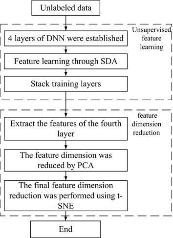
Fig. 8Comparison between two features and tool wear
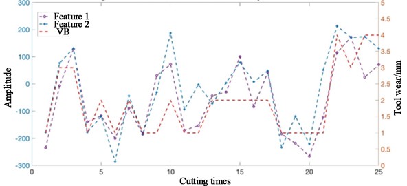
It can be seen from the figure that the feature proposed in this paper can well characterize the change of tool wear, which lays a good foundation for the classification of tool wear states in the future. These indications of tool wear can form new labeled data, as shown in Fig. 8, which provides a good database for further fine-tuning DNN parameters through back propagation.
3. Classification model of tool wear state using SDA
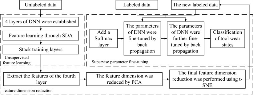
The tool wear state classification model can establish the mapping relationship between the feature matrix obtained from the original signal and the tool wear state. In this paper, a DNN network composed of 4 Sdas is used as the classification model of tool wear state. On this basis, Softmax layer is added to the output end of DNN to classify the tool wear state. The labeled data of the original data is fine-tuned into DNN parameters through backpropagation, and the new labeled data composed of primary reduction and secondary dimensionality reduction features is fine-tuned into DNN network parameters through backpropagation, as shown in Fig. 9.
In the figure, Softmax regression layer is a general logistic regression layer used to predict multi-objective classification problems. Suppose that the training data samples and labels with categories are known, where , , Softmax regression layer can be used to predict the probability that each input sample belongs to each category:
where 1,2..., , parameters of Softmax regression layer . The Softmax regression layer normalizes the probability distribution by ensuring that the sum of all probabilities equals one.
Fig. 9Tool wear condition classification model
The loss function of SoftMax regression layer is defined as follows:
where 1{·} denotes the indicator function, which is 1 when the condition is true and 0 otherwise. The parameters of the Softmax regression layer are constantly updated by decreasing the loss value.
After adding a Softmax regression layer to the output of the DNN, a small amount of labeled data reversely regulates the parameters of the DNN by reducing the error between the predicted and true values. Stochastic gradient descent based on backpropagation algorithm is used to continuously update the parameters of all hidden layers. The weights and biases are updated by the following equation:
where and are the weight and deviation matrix of the hidden layer, is the learning rate of the hidden layer, is the training data put in each time, is the containing sample point. DNN has the ability to classify tool wear state after two backpropagation fine-tuning.
4. Classification evaluation results and analysis of tool wear
Using the classification method of literature, the tool wear state is divided into four categories, as shown in Table 3. Where Ⅰ corresponds to the initial wear of the tool, Ⅱ and Ⅲ correspond to the normal wear of the tool, and Ⅳ corresponds to the sharp wear stage of the tool. In experimental data, the early wear and tear of the sample is more, the rapid wear of samples is less, to reduce the influence caused by the uneven sample, random forest classifier was used to solve this problem.
Table 3Tool wear condition classification
Tool wear condition classification | VB / mm |
Ⅰ | 0 ≤ VB < 0.2 |
Ⅱ | 0.2 ≤ VB < 0.4 |
Ⅲ | 0.4 ≤ VB < 0.6 |
Ⅳ | VB > 0.6 |
The ratio of training set and test set was set to 70 % and 30 %, and 10 experiments were performed on the model. After two fine-tuning of DNN parameters, the accuracy of its training set and test set is shown in Fig. 10.
Fig. 10Accuracy of tool wear condition classification of training data and data after two fine- tune
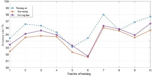
As can be seen from the figure, the accuracy of the training set is basically higher than 93 %, and the accuracy of the initial fine-tuning of DNN parameters is above 91 %. However, the accuracy of the new label data is improved, which indicates that the new label data, namely, the feature data after dimensionality reduction of features for many times, is more representative of the features of the original data. The same method is used to classify the tool wear state in other working conditions, and the accuracy is shown in Table 4.
From the experimental results in Table 4, we can see that both our proposed SDA method and random forest method perform well in identifying the tool wear state. This is because when the tool is seriously worn, the current signal of the spindle motor changes obviously, which can be shown by manually extracting signal features. Therefore, the recognition accuracy can reach 98.367 % by using SDA. However, when the wear difference is not large, such as working conditions A, D and E, the current signal of the spindle motor only changes weakly. Meanwhile, due to the change of processing parameters and the presence of noise signals, such weak changes cannot be distinguished by traditional feature extraction methods, so the recognition effect of random forest is poor. The recognition accuracy of using random forest is better than that of SDA when the amount of data is less, because random forest equalizes the data set. However, in the case of multiple data amounts, the wear state recognition accuracy of the method proposed in this paper is still 98.367 %, indicating that the method can adapt to the change of processing parameters and fully extract the characteristic information of signal characteristics.
Table 4Accuracy of tool wear condition in different cutting conditions
Working condition | The serial number | Random forest (literature) | SDA (method of this paper) |
A | 1, 9 | 86.154 | 83.612 |
B | 2, 12, 4, 10 | 97.273 | 98.367 |
C | 3, 11 | 93.333 | 94.245 |
D | 5, 16 | 85.833 | 83.215 |
E | 6, 8, 14, 15 | 86.667 | 90.487 |
F | 7, 13 | 88.571 | 84.560 |
The accuracy obtained by the SDA method is the accuracy after two fine-tuning of DNN parameters. It can be seen that the classification accuracy of the tool wear state of the SDA proposed in this paper is improved under working conditions B, C and E, while the tool wear accuracy is reduced under working conditions A, D and F. Through analysis, the reasons for the lower classification accuracy of tool wear state by the proposed method are as follows: (1) Although the feature matrix formed after feature extraction, feature selection and feature dimensionality reduction proposed in this paper can well represent the features of the original data, the DNN network has certain requirements on the amount of data, and the feature matrix undoubtedly reduces the amount of data, resulting in a poor performance of the advantages of DNN. (2) The data obtained from the experiment contains unbalanced samples of each tool wear state. In order to reduce the impact of uneven samples, this paper deleted some data containing a large number of samples, which also reduced the amount of data required by DNN. (3) The parameters of DNN network (such as the number of layers, the number of neurons in each layer, the learning rate, etc.) have an important impact on the prediction results, and the setting of these parameters is usually based on experience or a large number of experiments. Due to the limitations of experimental conditions, the optimal parameters of DNN network cannot be obtained.
To sum up, the recognition accuracy and accuracy of SDA have achieved good results under most working conditions, which fully embodies the advantages of the method proposed in this paper.
5. Conclusions
This paper presents an unsupervised deep neural network (DNN) tool condition monitoring based on stack denoising autoencoder (SDA), aiming at on-line monitoring and evaluation of tool wear in automatic machining. The signal collected by the current sensor is processed by the methods of feature extraction, feature selection and feature dimension reduction, and then the state recognition of the tool is realized by an unsupervised deep neural network (DNN) of stacked denoising autoencoder (SDA). The application effect of the model in monitoring tool wear condition was analyzed experimentally. The effectiveness and feasibility of the model in monitoring tool wear condition were verified through experiments, and the main conclusions were obtained as follows:
(1) The proposed idea of using the current sensor in the machine tool to obtain data overcomes the shortcomings of installing vibration sensors, acoustic emission sensors, force sensors and other sensors at present, and extends the adaptability of the method proposed in this paper. On the basis of the preliminary analysis of the data, the data of DC signal stabilization stage is used as the original data.
(2) Due to data loss and damage, data needs to be preprocessed. In the process of finding the indicator of tool wear state, the methods of feature extraction, feature selection and feature dimensionality reduction are integrated to ensure that the final feature matrix can fully represent the original data. Especially in the selection of feature dimension reduction method, the SDA method is introduced into the monitoring of tool wear state. The feature matrix after feature extraction and selection is preliminarily dimensionally reduced. On this basis, PCA and t-SNE are used to reduce the dimensionality of the features twice, and finally a simple two-dimensional feature matrix is obtained. The results show that the two characteristic matrices obtained are in good agreement with the change of tool wear.
(3) In the tool wear state evaluation, the deep neural network model of SDA was established by adding Softmax regression layer, the tool wear monitoring results were taken as the new labeled data, and the deep neural network parameters were fine adjusted by secondary backpropagation. The results show that compared with other studies, the evaluation accuracy of some results is improved. However, some results are not accurate. The reasons are analyzed and summarized to provide ideas for follow-up research.
References
-
S. Dutta, A. Kanwat, S. K. Pal, and R. Sen, “Correlation study of tool flank wear with machined surface texture in end milling,” Measurement, Vol. 46, No. 10, pp. 4249–4260, Dec. 2013, https://doi.org/10.1016/j.measurement.2013.07.015
-
C. Drouillet, J. Karandikar, C. Nath, A.-C. Journeaux, M. El Mansori, and T. Kurfess, “Tool life predictions in milling using spindle power with the neural network technique,” Journal of Manufacturing Processes, Vol. 22, pp. 161–168, Apr. 2016, https://doi.org/10.1016/j.jmapro.2016.03.010
-
G. F. Wang, Y. W. Yang, Y. C. Zhang, and Q. L. Xie, “Vibration sensor based tool condition monitoring using ν support vector machine and locality preserving projection,” Sensors and Actuators A: Physical, Vol. 209, pp. 24–32, Mar. 2014, https://doi.org/10.1016/j.sna.2014.01.004
-
Z. Yuqing, L. Xinfang, L. Fengping, S. Bingtao, and X. Wei, “An online damage identification approach for numerical control machine tools based on data fusion using vibration signals,” Journal of Vibration and Control, Vol. 21, No. 15, pp. 2925–2936, Nov. 2015, https://doi.org/10.1177/1077546314545097
-
M. Nouri, B. K. Fussell, B. L. Ziniti, and E. Linder, “Real-time tool wear monitoring in milling using a cutting condition independent method,” International Journal of Machine Tools and Manufacture, Vol. 89, pp. 1–13, Feb. 2015, https://doi.org/10.1016/j.ijmachtools.2014.10.011
-
K. Javed, R. Gouriveau, X. Li, and N. Zerhouni, “Tool wear monitoring and prognostics challenges: a comparison of connectionist methods toward an adaptive ensemble model,” Journal of Intelligent Manufacturing, Vol. 29, No. 8, pp. 1873–1890, Dec. 2018, https://doi.org/10.1007/s10845-016-1221-2
-
A. I. Azmi, “Monitoring of tool wear using measured machining forces and neuro-fuzzy modelling approaches during machining of GFRP composites,” Advances in Engineering Software, Vol. 82, pp. 53–64, Apr. 2015, https://doi.org/10.1016/j.advengsoft.2014.12.010
-
R. Koike, K. Ohnishi, and T. Aoyama, “A sensorless approach for tool fracture detection in milling by integrating multi-axial servo information,” CIRP Annals, Vol. 65, No. 1, pp. 385–388, 2016, https://doi.org/10.1016/j.cirp.2016.04.101
-
C.-L. Yen, M.-C. Lu, and J.-L. Chen, “Applying the self-organization feature map (SOM) algorithm to AE-based tool wear monitoring in micro-cutting,” Mechanical Systems and Signal Processing, Vol. 34, No. 1-2, pp. 353–366, Jan. 2013, https://doi.org/10.1016/j.ymssp.2012.05.001
-
V. A. Pechenin, A. I. Khaimovich, A. I. Kondratiev, and M. A. Bolotov, “Method of controlling cutting tool wear based on signal analysis of acoustic emission for milling,” Procedia Engineering, Vol. 176, pp. 246–252, 2017, https://doi.org/10.1016/j.proeng.2017.02.294
-
K. Zhu and B. Vogel-Heuser, “Sparse representation and its applications in micro-milling condition monitoring: noise separation and tool condition monitoring,” The International Journal of Advanced Manufacturing Technology, Vol. 70, No. 1-4, pp. 185–199, Jan. 2014, https://doi.org/10.1007/s00170-013-5258-5
-
M. Luo, H. Luo, D. Axinte, D. Liu, J. Mei, and Z. Liao, “A wireless instrumented milling cutter system with embedded PVDF sensors,” Mechanical Systems and Signal Processing, Vol. 110, pp. 556–568, Sep. 2018, https://doi.org/10.1016/j.ymssp.2018.03.040
-
N. Ghosh et al., “Estimation of tool wear during CNC milling using neural network-based sensor fusion,” Mechanical Systems and Signal Processing, Vol. 21, No. 1, pp. 466–479, Jan. 2007, https://doi.org/10.1016/j.ymssp.2005.10.010
-
M. Rizal, J. A. Ghani, M. Zaki Nuawi, and C. Hassan Che Haron, “A Review of Sensor System and Application in Milling Process for Tool Condition Monitoring,” Research Journal of Applied Sciences, Engineering and Technology, Vol. 7, No. 10, pp. 2083–2097, Mar. 2014, https://doi.org/10.19026/rjaset.7.502
-
S.-L. Chen and Y. W. Jen, “Data fusion neural network for tool condition monitoring in CNC milling machining,” International Journal of Machine Tools and Manufacture, Vol. 40, No. 3, pp. 381–400, Feb. 2000, https://doi.org/10.1016/s0890-6955(99)00066-8
-
S. Barua, M. M. Islam, X. Yao, and K. Murase, “MWMOTE--majority weighted minority oversampling technique for imbalanced data set learning,” IEEE Transactions on Knowledge and Data Engineering, Vol. 26, No. 2, pp. 405–425, Feb. 2014, https://doi.org/10.1109/tkde.2012.232
-
J. Karandikar, T. Mcleay, S. Turner, and T. Schmitz, “Tool wear monitoring using naïve Bayes classifiers,” The International Journal of Advanced Manufacturing Technology, Vol. 77, No. 9-12, pp. 1613–1626, Apr. 2015, https://doi.org/10.1007/s00170-014-6560-6
-
T. Liu, Q. Wang, and W. Wang, “Micro-milling tool wear monitoring via nonlinear cutting force model,” Micromachines, Vol. 13, No. 6, p. 943, Jun. 2022, https://doi.org/10.3390/mi13060943
-
N. Seemuang, T. Mcleay, and T. Slatter, “Using spindle noise to monitor tool wear in a turning process,” The International Journal of Advanced Manufacturing Technology, Vol. 86, No. 9-12, pp. 2781–2790, Oct. 2016, https://doi.org/10.1007/s00170-015-8303-8
-
X. Zhang, Y. Gao, Z. Guo, W. Zhang, J. Yin, and W. Zhao, “Physical model-based tool wear and breakage monitoring in milling process,” Mechanical Systems and Signal Processing, Vol. 184, p. 109641, Feb. 2023, https://doi.org/10.1016/j.ymssp.2022.109641
-
E. Kannatey-Asibu, J. Yum, and T. H. Kim, “Monitoring tool wear using classifier fusion,” Mechanical Systems and Signal Processing, Vol. 85, pp. 651–661, Feb. 2017, https://doi.org/10.1016/j.ymssp.2016.08.035
Cited by
About this article

The authors have not disclosed any funding.
The datasets generated during and/or analyzed during the current study are available from the corresponding author on reasonable request.
Jingjing Gao conceived the idea. Jingjing Gao and Jing Liu performed all the experiments. Jingjing Gao drafted the manuscript, and Jingjing Gao, Xinli Yu interpreted, discussed and edited the manuscript. Jingjing Gao and Xinli Yu finalized the manuscript, including preparing the detailed response letter. Jingjing Gao supervised the work.
The authors declare that they have no conflict of interest.
